Signals Analysis

---

---

Analogy Between Vectors and Signals

There is a perfect analogy between vectors and signals.

Vector

A vector contains magnitude and direction. The name of the vector is denoted by bold face type and their magnitude is denoted by light face type.

Example: V is a vector with magnitude V. Consider two vectors V₁ and V₂ as shown in the following diagram. Let the component of V₁ along with V₂ is given by C₁₂V₂. The component of a vector V₁ along with the vector V₂ can obtained by taking a perpendicular from the end of V₁ to the vector V₂ as shown in diagram:

The vector V₁ can be expressed in terms of vector V₂

V₁= C₁₂V₂ + V_e

Where Ve is the error vector.

But this is not the only way of expressing vector V₁ in terms of V₂. The alternate possibilities are:

The error signal is minimum for large component value. If C₁₂=0, then two signals are said to be orthogonal.

Dot Product of Two Vectors

V₁ . V₂ = V₁.V₂ cosθ

θ = Angle between V1 and V2

V₁ . V₂ =V₂.V₁

The components of V₁ alog_n V₂ = V₁ Cos θ = $V1.V2 \over V2$

From the diagram, components of V₁ alog_n V₂ = C ₁₂ V₂

$$V_1.V_2 \over V_2 = C_12\,V_2$$

$$ \Rightarrow C_{12} = {V_1.V_2 \over V_2}$$

Signal

The concept of orthogonality can be applied to signals. Let us consider two signals f₁(t) and f₂(t). Similar to vectors, you can approximate f₁(t) in terms of f₂(t) as

f₁(t) = C₁₂ f₂(t) + f_e(t) for (t₁ 2)

$ \Rightarrow $ f_e(t) = f₁(t) C₁₂ f₂(t)

One possible way of minimizing the error is integrating over the interval t₁ to t₂.

$${1 \over {t_2 - t_1}} \int_{t_1}^{t_2} [f_e (t)] dt$$

$${1 \over {t_2 - t_1}} \int_{t_1}^{t_2} [f_1(t) - C_{12}f_2(t)]dt $$

However, this step also does not reduce the error to appreciable extent. This can be corrected by taking the square of error function.

$\varepsilon = {1 \over {t_2 - t_1}} \int_{t_1}^{t_2} [f_e (t)]^2 dt$

$\Rightarrow {1 \over {t_2 - t_1}} \int_{t_1}^{t_2} [f_e (t) - C_{12}f_2]^2 dt $

Where ε is the mean square value of error signal. The value of C₁₂ which minimizes the error, you need to calculate ${d\varepsilon \over dC_{12} } = 0 $

$\Rightarrow {d \over dC_{12} } [ {1 \over t_2 - t_1 } \int_{t_1}^{t_2} [f_1 (t) - C_{12} f_2 (t)]^2 dt]= 0 $

$\Rightarrow {1 \over {t_2 - t_1}} \int_{t_1}^{t_2} [ {d \over dC_{12} } f_{1}^2(t) - {d \over dC_{12} } 2f_1(t)C_{12}f_2(t)+ {d \over dC_{12} } f_{2}^{2} (t) C_{12}^2 ] dt =0 $

Derivative of the terms which do not have C12 term are zero.

$\Rightarrow \int_{t_1}^{t_2} - 2f_1(t) f_2(t) dt + 2C_{12}\int_{t_1}^{t_2}[f_{2}^{2} (t)]dt = 0 $

If $C_{12} = {{\int_{t_1}^{t_2}f_1(t)f_2(t)dt } \over {\int_{t_1}^{t_2} f_{2}^{2} (t)dt }} $ component is zero, then two signals are said to be orthogonal.

Put C₁₂ = 0 to get condition for orthogonality.

0 = $ {{\int_{t_1}^{t_2}f_1(t)f_2(t)dt } \over {\int_{t_1}^{t_2} f_{2}^{2} (t)dt }} $

$$ \int_{t_1}^{t_2} f_1 (t)f_2(t) dt = 0 $$

Orthogonal Vector Space

A complete set of orthogonal vectors is referred to as orthogonal vector space. Consider a three dimensional vector space as shown below:

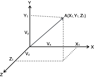
Consider a vector A at a point (X₁, Y₁, Z₁). Consider three unit vectors (V_X, V_Y, V_Z) in the direction of X, Y, Z axis respectively. Since these unit vectors are mutually orthogonal, it satisfies that

$$V_X. V_X= V_Y. V_Y= V_Z. V_Z = 1 $$

$$V_X. V_Y= V_Y. V_Z= V_Z. V_X = 0 $$

You can write above conditions as

$$V_a . V_b = \left\{ \begin{array}{l l} 1 & \quad a = b \\ 0 & \quad a \neq b \end{array} \right. $$

The vector A can be represented in terms of its components and unit vectors as

$A = X_1 V_X + Y_1 V_Y + Z_1 V_Z................(1) $

Any vectors in this three dimensional space can be represented in terms of these three unit vectors only.

If you consider n dimensional space, then any vector A in that space can be represented as

$ A = X_1 V_X + Y_1 V_Y + Z_1 V_Z+...+ N_1V_N.....(2) $

As the magnitude of unit vectors is unity for any vector A

The component of A along x axis = A.V_X

The component of A along Y axis = A.V_Y

The component of A along Z axis = A.V_Z

Similarly, for n dimensional space, the component of A along some G axis

$= A.VG...............(3)$

Substitute equation 2 in equation 3.

$\Rightarrow CG= (X_1 V_X + Y_1 V_Y + Z_1 V_Z +...+G_1 V_G...+ N_1V_N)V_G$

$= X_1 V_X V_G + Y_1 V_Y V_G + Z_1 V_Z V_G +...+ G_1V_G V_G...+ N_1V_N V_G$

$= G_1 \,\,\,\,\, \text{since } V_G V_G=1$

$If V_G V_G \neq 1 \,\,\text{i.e.} V_G V_G= k$

$AV_G = G_1V_G V_G= G_1K$

$G_1 = {(AV_G) \over K}$

Orthogonal Signal Space

Let us consider a set of n mutually orthogonal functions x₁(t), x₂(t)... x_n(t) over the interval t₁ to t₂. As these functions are orthogonal to each other, any two signals x_j(t), x_k(t) have to satisfy the orthogonality condition. i.e.

$$\int_{t_1}^{t_2} x_j(t)x_k(t)dt = 0 \,\,\, \text{where}\, j \neq k$$

$$\text{Let} \int_{t_1}^{t_2}x_{k}^{2}(t)dt = k_k $$

Let a function f(t), it can be approximated with this orthogonal signal space by adding the components along mutually orthogonal signals i.e.

$\,\,\,f(t) = C_1x_1(t) + C_2x_2(t) + ... + C_nx_n(t) + f_e(t) $

$\quad\quad=\Sigma_{r=1}^{n} C_rx_r (t) $

$\,\,\,f(t) = f(t) - \Sigma_{r=1}^n C_rx_r (t) $

Mean sqaure error $ \varepsilon = {1 \over t_2 - t_2 } \int_{t_1}^{t_2} [ f_e(t)]^2 dt$

$$ = {1 \over t_2 - t_2 } \int_{t_1}^{t_2} [ f[t] - \sum_{r=1}^{n} C_rx_r(t) ]^2 dt $$

The component which minimizes the mean square error can be found by

$$ {d\varepsilon \over dC_1} = {d\varepsilon \over dC_2} = ... = {d\varepsilon \over dC_k} = 0 $$

Let us consider ${d\varepsilon \over dC_k} = 0 $

$${d \over dC_k}[ {1 \over t_2 - t_1} \int_{t_1}^{t_2} [ f(t) - \Sigma_{r=1}^n C_rx_r(t)]^2 dt] = 0 $$

All terms that do not contain C_k is zero. i.e. in summation, r=k term remains and all other terms are zero.

$$\int_{t_1}^{t_2} - 2 f(t)x_k(t)dt + 2C_k \int_{t_1}^{t_2} [x_k^2 (t)] dt=0 $$

$$\Rightarrow C_k = {{\int_{t_1}^{t_2}f(t)x_k(t)dt} \over {int_{t_1}^{t_2} x_k^2 (t)dt}} $$

$$\Rightarrow \int_{t_1}^{t_2} f(t)x_k(t)dt = C_kK_k $$

Mean Square Error

The average of square of error function f_e(t) is called as mean square error. It is denoted by ε (epsilon).

.

$\varepsilon = {1 \over t_2 - t_1 } \int_{t_1}^{t_2} [f_e (t)]^2dt$

$\,\,\,\,= {1 \over t_2 - t_1 } \int_{t_1}^{t_2} [f_e (t) - \Sigma_{r=1}^n C_rx_r(t)]^2 dt $

$\,\,\,\,= {1 \over t_2 - t_1 } [ \int_{t_1}^{t_2} [f_e^2 (t) ]dt + \Sigma_{r=1}^{n} C_r^2 \int_{t_1}^{t_2} x_r^2 (t) dt - 2 \Sigma_{r=1}^{n} C_r \int_{t_1}^{t_2} x_r (t)f(t)dt$

You know that $C_{r}^{2} \int_{t_1}^{t_2} x_r^2 (t)dt = C_r \int_{t_1}^{t_2} x_r (t)f(d)dt = C_r^2 K_r $

$\varepsilon = {1 \over t_2 - t_1 } [ \int_{t_1}^{t_2} [f^2 (t)] dt + \Sigma_{r=1}^{n} C_r^2 K_r - 2 \Sigma_{r=1}^{n} C_r^2 K_r] $

$\,\,\,\,= {1 \over t_2 - t_1 } [\int_{t_1}^{t_2} [f^2 (t)] dt - \Sigma_{r=1}^{n} C_r^2 K_r ] $

$\, \therefore \varepsilon = {1 \over t_2 - t_1 } [\int_{t_1}^{t_2} [f^2 (t)] dt + (C_1^2 K_1 + C_2^2 K_2 + ... + C_n^2 K_n)] $

The above equation is used to evaluate the mean square error.

Closed and Complete Set of Orthogonal Functions

Let us consider a set of n mutually orthogonal functions x₁(t), x₂(t)...x_n(t) over the interval t₁ to t₂. This is called as closed and complete set when there exist no function f(t) satisfying the condition $\int_{t_1}^{t_2} f(t)x_k(t)dt = 0 $

If this function is satisfying the equation $\int_{t_1}^{t_2} f(t)x_k(t)dt=0 \,\, \text{for}\, k = 1,2,..$ then f(t) is said to be orthogonal to each and every function of orthogonal set. This set is incomplete without f(t). It becomes closed and complete set when f(t) is included.

f(t) can be approximated with this orthogonal set by adding the components along mutually orthogonal signals i.e.

$$f(t) = C_1 x_1(t) + C_2 x_2(t) + ... + C_n x_n(t) + f_e(t) $$

If the infinite series $C_1 x_1(t) + C_2 x_2(t) + ... + C_n x_n(t)$ converges to f(t) then mean square error is zero.

Orthogonality in Complex Functions

If f₁(t) and f₂(t) are two complex functions, then f₁(t) can be expressed in terms of f₂(t) as

$f_1(t) = C_{12}f_2(t) \,\,\,\,\,\,\,\,$ ..with negligible error

Where $C_{12} = {{\int_{t_1}^{t_2} f_1(t)f_2^*(t)dt} \over { \int_{t_1}^{t_2} |f_2(t)|^2 dt}} $

Where $f_2^* (t)$ = complex conjugate of f₂(t).

If f₁(t) and f₂(t) are orthogonal then C₁₂ = 0

$$ {\int_{t_1}^{t_2} f_1 (t) f_2^*(t) dt \over \int_{t_1}^{t_2} |f_2 (t) |^2 dt} = 0 $$

$$\Rightarrow \int_{t_1}^{t_2} f_1 (t) f_2^* (dt) = 0$$

The above equation represents orthogonality condition in complex functions.