- Signals & Systems Home
- Signals & Systems Overview
- Introduction
- Signals Basic Types
- Signals Classification
- Signals Basic Operations
- Systems Classification
- Types of Signals
- Representation of a Discrete Time Signal
- Continuous-Time Vs Discrete-Time Sinusoidal Signal
- Even and Odd Signals
- Properties of Even and Odd Signals
- Periodic and Aperiodic Signals
- Unit Step Signal
- Unit Ramp Signal
- Unit Parabolic Signal
- Energy Spectral Density
- Unit Impulse Signal
- Power Spectral Density
- Properties of Discrete Time Unit Impulse Signal
- Real and Complex Exponential Signals
- Addition and Subtraction of Signals
- Amplitude Scaling of Signals
- Multiplication of Signals
- Time Scaling of Signals
- Time Shifting Operation on Signals
- Time Reversal Operation on Signals
- Even and Odd Components of a Signal
- Energy and Power Signals
- Power of an Energy Signal over Infinite Time
- Energy of a Power Signal over Infinite Time
- Causal, Non-Causal, and Anti-Causal Signals
- Rectangular, Triangular, Signum, Sinc, and Gaussian Functions
- Signals Analysis
- Types of Systems
- What is a Linear System?
- Time Variant and Time-Invariant Systems
- Linear and Non-Linear Systems
- Static and Dynamic System
- Causal and Non-Causal System
- Stable and Unstable System
- Invertible and Non-Invertible Systems
- Linear Time-Invariant Systems
- Transfer Function of LTI System
- Properties of LTI Systems
- Response of LTI System
- Fourier Series
- Fourier Series
- Fourier Series Representation of Periodic Signals
- Fourier Series Types
- Trigonometric Fourier Series Coefficients
- Exponential Fourier Series Coefficients
- Complex Exponential Fourier Series
- Relation between Trigonometric & Exponential Fourier Series
- Fourier Series Properties
- Properties of Continuous-Time Fourier Series
- Time Differentiation and Integration Properties of Continuous-Time Fourier Series
- Time Shifting, Time Reversal, and Time Scaling Properties of Continuous-Time Fourier Series
- Linearity and Conjugation Property of Continuous-Time Fourier Series
- Multiplication or Modulation Property of Continuous-Time Fourier Series
- Convolution Property of Continuous-Time Fourier Series
- Convolution Property of Fourier Transform
- Parseval’s Theorem in Continuous Time Fourier Series
- Average Power Calculations of Periodic Functions Using Fourier Series
- GIBBS Phenomenon for Fourier Series
- Fourier Cosine Series
- Trigonometric Fourier Series
- Derivation of Fourier Transform from Fourier Series
- Difference between Fourier Series and Fourier Transform
- Wave Symmetry
- Even Symmetry
- Odd Symmetry
- Half Wave Symmetry
- Quarter Wave Symmetry
- Fourier Transform
- Fourier Transforms
- Fourier Transforms Properties
- Fourier Transform – Representation and Condition for Existence
- Properties of Continuous-Time Fourier Transform
- Table of Fourier Transform Pairs
- Linearity and Frequency Shifting Property of Fourier Transform
- Modulation Property of Fourier Transform
- Time-Shifting Property of Fourier Transform
- Time-Reversal Property of Fourier Transform
- Time Scaling Property of Fourier Transform
- Time Differentiation Property of Fourier Transform
- Time Integration Property of Fourier Transform
- Frequency Derivative Property of Fourier Transform
- Parseval’s Theorem & Parseval’s Identity of Fourier Transform
- Fourier Transform of Complex and Real Functions
- Fourier Transform of a Gaussian Signal
- Fourier Transform of a Triangular Pulse
- Fourier Transform of Rectangular Function
- Fourier Transform of Signum Function
- Fourier Transform of Unit Impulse Function
- Fourier Transform of Unit Step Function
- Fourier Transform of Single-Sided Real Exponential Functions
- Fourier Transform of Two-Sided Real Exponential Functions
- Fourier Transform of the Sine and Cosine Functions
- Fourier Transform of Periodic Signals
- Conjugation and Autocorrelation Property of Fourier Transform
- Duality Property of Fourier Transform
- Analysis of LTI System with Fourier Transform
- Relation between Discrete-Time Fourier Transform and Z Transform
- Convolution and Correlation
- Convolution in Signals and Systems
- Convolution and Correlation
- Correlation in Signals and Systems
- System Bandwidth vs Signal Bandwidth
- Time Convolution Theorem
- Frequency Convolution Theorem
- Energy Spectral Density and Autocorrelation Function
- Autocorrelation Function of a Signal
- Cross Correlation Function and its Properties
- Detection of Periodic Signals in the Presence of Noise (by Autocorrelation)
- Detection of Periodic Signals in the Presence of Noise (by Cross-Correlation)
- Autocorrelation Function and its Properties
- PSD and Autocorrelation Function
- Sampling
- Signals Sampling Theorem
- Nyquist Rate and Nyquist Interval
- Signals Sampling Techniques
- Effects of Undersampling (Aliasing) and Anti Aliasing Filter
- Different Types of Sampling Techniques
- Laplace Transform
- Laplace Transforms
- Common Laplace Transform Pairs
- Laplace Transform of Unit Impulse Function and Unit Step Function
- Laplace Transform of Sine and Cosine Functions
- Laplace Transform of Real Exponential and Complex Exponential Functions
- Laplace Transform of Ramp Function and Parabolic Function
- Laplace Transform of Damped Sine and Cosine Functions
- Laplace Transform of Damped Hyperbolic Sine and Cosine Functions
- Laplace Transform of Periodic Functions
- Laplace Transform of Rectifier Function
- Laplace Transforms Properties
- Linearity Property of Laplace Transform
- Time Shifting Property of Laplace Transform
- Time Scaling and Frequency Shifting Properties of Laplace Transform
- Time Differentiation Property of Laplace Transform
- Time Integration Property of Laplace Transform
- Time Convolution and Multiplication Properties of Laplace Transform
- Initial Value Theorem of Laplace Transform
- Final Value Theorem of Laplace Transform
- Parseval's Theorem for Laplace Transform
- Laplace Transform and Region of Convergence for right sided and left sided signals
- Laplace Transform and Region of Convergence of Two Sided and Finite Duration Signals
- Circuit Analysis with Laplace Transform
- Step Response and Impulse Response of Series RL Circuit using Laplace Transform
- Step Response and Impulse Response of Series RC Circuit using Laplace Transform
- Step Response of Series RLC Circuit using Laplace Transform
- Solving Differential Equations with Laplace Transform
- Difference between Laplace Transform and Fourier Transform
- Difference between Z Transform and Laplace Transform
- Relation between Laplace Transform and Z-Transform
- Relation between Laplace Transform and Fourier Transform
- Laplace Transform – Time Reversal, Conjugation, and Conjugate Symmetry Properties
- Laplace Transform – Differentiation in s Domain
- Laplace Transform – Conditions for Existence, Region of Convergence, Merits & Demerits
- Z Transform
- Z-Transforms (ZT)
- Common Z-Transform Pairs
- Z-Transform of Unit Impulse, Unit Step, and Unit Ramp Functions
- Z-Transform of Sine and Cosine Signals
- Z-Transform of Exponential Functions
- Z-Transforms Properties
- Properties of ROC of the Z-Transform
- Z-Transform and ROC of Finite Duration Sequences
- Conjugation and Accumulation Properties of Z-Transform
- Time Shifting Property of Z Transform
- Time Reversal Property of Z Transform
- Time Expansion Property of Z Transform
- Differentiation in z Domain Property of Z Transform
- Initial Value Theorem of Z-Transform
- Final Value Theorem of Z Transform
- Solution of Difference Equations Using Z Transform
- Long Division Method to Find Inverse Z Transform
- Partial Fraction Expansion Method for Inverse Z-Transform
- What is Inverse Z Transform?
- Inverse Z-Transform by Convolution Method
- Transform Analysis of LTI Systems using Z-Transform
- Convolution Property of Z Transform
- Correlation Property of Z Transform
- Multiplication by Exponential Sequence Property of Z Transform
- Multiplication Property of Z Transform
- Residue Method to Calculate Inverse Z Transform
- System Realization
- Cascade Form Realization of Continuous-Time Systems
- Direct Form-I Realization of Continuous-Time Systems
- Direct Form-II Realization of Continuous-Time Systems
- Parallel Form Realization of Continuous-Time Systems
- Causality and Paley Wiener Criterion for Physical Realization
- Discrete Fourier Transform
- Discrete-Time Fourier Transform
- Properties of Discrete Time Fourier Transform
- Linearity, Periodicity, and Symmetry Properties of Discrete-Time Fourier Transform
- Time Shifting and Frequency Shifting Properties of Discrete Time Fourier Transform
- Inverse Discrete-Time Fourier Transform
- Time Convolution and Frequency Convolution Properties of Discrete-Time Fourier Transform
- Differentiation in Frequency Domain Property of Discrete Time Fourier Transform
- Parseval’s Power Theorem
- Miscellaneous Concepts
- What is Mean Square Error?
- What is Fourier Spectrum?
- Region of Convergence
- Hilbert Transform
- Properties of Hilbert Transform
- Symmetric Impulse Response of Linear-Phase System
- Filter Characteristics of Linear Systems
- Characteristics of an Ideal Filter (LPF, HPF, BPF, and BRF)
- Zero Order Hold and its Transfer Function
- What is Ideal Reconstruction Filter?
- What is the Frequency Response of Discrete Time Systems?
- Basic Elements to Construct the Block Diagram of Continuous Time Systems
- BIBO Stability Criterion
- BIBO Stability of Discrete-Time Systems
- Distortion Less Transmission
- Distortionless Transmission through a System
- Rayleigh’s Energy Theorem
Signals and Systems - Quick Guide
What is Signal?
Signal is a time varying physical phenomenon which is intended to convey information.
OR
Signal is a function of time.
OR
Signal is a function of one or more independent variables, which contain some information.
Example: voice signal, video signal, signals on telephone wires etc.
Note: Noise is also a signal, but the information conveyed by noise is unwanted hence it is considered as undesirable.

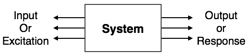
What is System?
System is a device or combination of devices, which can operate on signals and produces corresponding response. Input to a system is called as excitation and output from it is called as response.
For one or more inputs, the system can have one or more outputs.
Example: Communication System
Signals Basic Types
Here are a few basic signals:
Unit Step Function
Unit step function is denoted by u(t). It is defined as u(t) = $\left\{\begin{matrix}1 & t \geqslant 0\\ 0 & t<0 \end{matrix}\right.$

- It is used as best test signal.
- Area under unit step function is unity.
Unit Impulse Function
Impulse function is denoted by δ(t). and it is defined as δ(t) = $\left\{\begin{matrix}1 & t = 0\\ 0 & t\neq 0 \end{matrix}\right.$
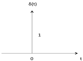
$$ \int_{-\infty}^{\infty} δ(t)dt=u (t)$$
$$ \delta(t) = {du(t) \over dt } $$
Ramp Signal
Ramp signal is denoted by r(t), and it is defined as r(t) = $\left\{\begin {matrix}t & t\geqslant 0\\ 0 & t < 0 \end{matrix}\right. $

$$ \int u(t) = \int 1 = t = r(t) $$
$$ u(t) = {dr(t) \over dt} $$
Area under unit ramp is unity.
Parabolic Signal
Parabolic signal can be defined as x(t) = $\left\{\begin{matrix} t^2/2 & t \geqslant 0\\ 0 & t < 0 \end{matrix}\right.$

$$\iint u(t)dt = \int r(t)dt = \int t dt = {t^2 \over 2} = parabolic signal $$
$$ \Rightarrow u(t) = {d^2x(t) \over dt^2} $$
$$ \Rightarrow r(t) = {dx(t) \over dt} $$
Signum Function
Signum function is denoted as sgn(t). It is defined as sgn(t) = $ \left\{\begin{matrix}1 & t>0\\ 0 & t=0\\ -1 & t<0 \end{matrix}\right. $

Exponential Signal
Exponential signal is in the form of x(t) = $e^{\alpha t}$.
The shape of exponential can be defined by $\alpha$.
Case i: if $\alpha$ = 0 $\to$ x(t) = $e^0$ = 1

Case ii: if $\alpha$ < 0 i.e. -ve then x(t) = $e^{-\alpha t}$. The shape is called decaying exponential.

Case iii: if $\alpha$ > 0 i.e. +ve then x(t) = $e^{\alpha t}$. The shape is called raising exponential.

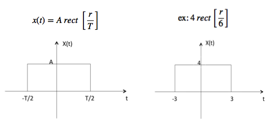
Rectangular Signal
Let it be denoted as x(t) and it is defined as
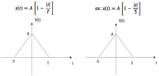
Triangular Signal
Let it be denoted as x(t)
Sinusoidal Signal
Sinusoidal signal is in the form of x(t) = A cos(${w}_{0}\,\pm \phi$) or A sin(${w}_{0}\,\pm \phi$)
Where T0 = $ 2\pi \over {w}_{0} $
Sinc Function
It is denoted as sinc(t) and it is defined as sinc
$$ (t) = {sin \pi t \over \pi t} $$
$$ = 0\, \text{for t} = \pm 1, \pm 2, \pm 3 ... $$

Sampling Function
It is denoted as sa(t) and it is defined as
$$sa(t) = {sin t \over t}$$
$$= 0 \,\, \text{for t} = \pm \pi,\, \pm 2 \pi,\, \pm 3 \pi \,... $$

Signals Classification
Signals are classified into the following categories:
Continuous Time and Discrete Time Signals
Deterministic and Non-deterministic Signals
Even and Odd Signals
Periodic and Aperiodic Signals
Energy and Power Signals
Real and Imaginary Signals
Continuous Time and Discrete Time Signals
A signal is said to be continuous when it is defined for all instants of time.
A signal is said to be discrete when it is defined at only discrete instants of time/

Deterministic and Non-deterministic Signals
A signal is said to be deterministic if there is no uncertainty with respect to its value at any instant of time. Or, signals which can be defined exactly by a mathematical formula are known as deterministic signals.

A signal is said to be non-deterministic if there is uncertainty with respect to its value at some instant of time. Non-deterministic signals are random in nature hence they are called random signals. Random signals cannot be described by a mathematical equation. They are modelled in probabilistic terms.

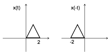
Even and Odd Signals
A signal is said to be even when it satisfies the condition x(t) = x(-t)
Example 1: t2, t4 cost etc.
Let x(t) = t2
x(-t) = (-t)2 = t2 = x(t)
$\therefore, $ t2 is even function
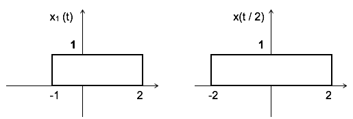
Example 2: As shown in the following diagram, rectangle function x(t) = x(-t) so it is also even function.

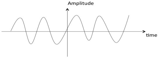
A signal is said to be odd when it satisfies the condition x(t) = -x(-t)
Example: t, t3 ... And sin t
Let x(t) = sin t
x(-t) = sin(-t) = -sin t = -x(t)
$\therefore, $ sin t is odd function.
Any function (t) can be expressed as the sum of its even function e(t) and odd function o(t).
(t ) = e(t ) + 0(t )
where
e(t ) = ½[(t ) +(-t )]
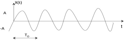
Periodic and Aperiodic Signals
A signal is said to be periodic if it satisfies the condition x(t) = x(t + T) or x(n) = x(n + N).
Where
T = fundamental time period,
1/T = f = fundamental frequency.
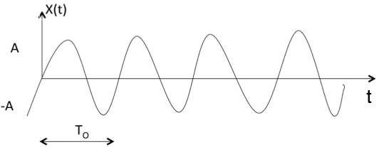
The above signal will repeat for every time interval T0 hence it is periodic with period T0.
Energy and Power Signals
A signal is said to be energy signal when it has finite energy.
$$\text{Energy}\, E = \int_{-\infty}^{\infty} x^2\,(t)dt$$
A signal is said to be power signal when it has finite power.
$$\text{Power}\, P = \lim_{T \to \infty}\,{1\over2T}\,\int_{-T}^{T}\,x^2(t)dt$$
NOTE:A signal cannot be both, energy and power simultaneously. Also, a signal may be neither energy nor power signal.
Power of energy signal = 0
Energy of power signal = ∞
Real and Imaginary Signals
A signal is said to be real when it satisfies the condition x(t) = x*(t)
A signal is said to be odd when it satisfies the condition x(t) = -x*(t)
Example:
If x(t)= 3 then x*(t)=3*=3 here x(t) is a real signal.
If x(t)= 3j then x*(t)=3j* = -3j = -x(t) hence x(t) is a odd signal.
Note: For a real signal, imaginary part should be zero. Similarly for an imaginary signal, real part should be zero.
Signals Basic Operations
There are two variable parameters in general:
- Amplitude
- Time
The following operation can be performed with amplitude:
Amplitude Scaling
C x(t) is a amplitude scaled version of x(t) whose amplitude is scaled by a factor C.

Addition
Addition of two signals is nothing but addition of their corresponding amplitudes. This can be best explained by using the following example:
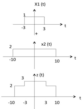
As seen from the diagram above,
-10 < t < -3 amplitude of z(t) = x1(t) + x2(t) = 0 + 2 = 2
-3 < t < 3 amplitude of z(t) = x1(t) + x2(t) = 1 + 2 = 3
3 < t < 10 amplitude of z(t) = x1(t) + x2(t) = 0 + 2 = 2
Subtraction
subtraction of two signals is nothing but subtraction of their corresponding amplitudes. This can be best explained by the following example:
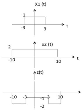
As seen from the diagram above,
- -10 < t < -3 amplitude of z (t) = x1(t) - x2(t) = 0 - 2 = -2
- -3 < t < 3 amplitude of z (t) = x1(t) - x2(t) = 1 - 2 = -1
- 3 < t < 10 amplitude of z (t) = x1(t) + x2(t) = 0 - 2 = -2
Multiplication
Multiplication of two signals is nothing but multiplication of their corresponding amplitudes. This can be best explained by the following example:
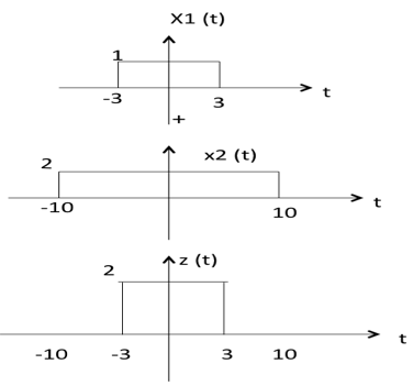
As seen from the diagram above,
-10 < t < -3 amplitude of z (t) = x1(t) x2(t) = 0 2 = 0
-3 < t < 3 amplitude of z (t) = x1(t) x2(t) = 1 2 = 2
3 < t < 10 amplitude of z (t) = x1(t) x2(t) = 0 2 = 0
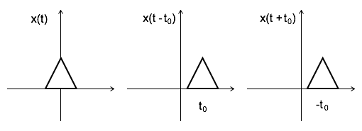
Time Shifting
x(t $\pm$ t0) is time shifted version of the signal x(t).
x (t + t0) $\to$ negative shift
x (t - t0) $\to$ positive shift
Time Scaling
x(At) is time scaled version of the signal x(t). where A is always positive.
|A| > 1 $\to$ Compression of the signal
|A| < 1 $\to$ Expansion of the signal
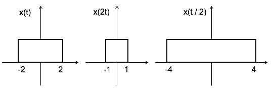
Note: u(at) = u(t) time scaling is not applicable for unit step function.
Time Reversal
x(-t) is the time reversal of the signal x(t).
Systems Classification
Systems are classified into the following categories:
- linear and Non-linear Systems
- Time Variant and Time Invariant Systems
- linear Time variant and linear Time invariant systems
- Static and Dynamic Systems
- Causal and Non-causal Systems
- Invertible and Non-Invertible Systems
- Stable and Unstable Systems
linear and Non-linear Systems
A system is said to be linear when it satisfies superposition and homogenate principles. Consider two systems with inputs as x1(t), x2(t), and outputs as y1(t), y2(t) respectively. Then, according to the superposition and homogenate principles,
T [a1 x1(t) + a2 x2(t)] = a1 T[x1(t)] + a2 T[x2(t)]
$\therefore, $ T [a1 x1(t) + a2 x2(t)] = a1 y1(t) + a2 y2(t)
From the above expression, is clear that response of overall system is equal to response of individual system.
Example:
(t) = x2(t)
Solution:
y1 (t) = T[x1(t)] = x12(t)
y2 (t) = T[x2(t)] = x22(t)
T [a1 x1(t) + a2 x2(t)] = [ a1 x1(t) + a2 x2(t)]2
Which is not equal to a1 y1(t) + a2 y2(t). Hence the system is said to be non linear.
Time Variant and Time Invariant Systems
A system is said to be time variant if its input and output characteristics vary with time. Otherwise, the system is considered as time invariant.
The condition for time invariant system is:
y (n , t) = y(n-t)
The condition for time variant system is:
y (n , t) $\neq$ y(n-t)
Where y (n , t) = T[x(n-t)] = input change
y (n-t) = output change
Example:
y(n) = x(-n)
y(n, t) = T[x(n-t)] = x(-n-t)
y(n-t) = x(-(n-t)) = x(-n + t)
$\therefore$ y(n, t) y(n-t). Hence, the system is time variant.
linear Time variant (LTV) and linear Time Invariant (LTI) Systems
If a system is both linear and time variant, then it is called linear time variant (LTV) system.
If a system is both linear and time Invariant then that system is called linear time invariant (LTI) system.
Static and Dynamic Systems
Static system is memory-less whereas dynamic system is a memory system.
Example 1: y(t) = 2 x(t)
For present value t=0, the system output is y(0) = 2x(0). Here, the output is only dependent upon present input. Hence the system is memory less or static.
Example 2: y(t) = 2 x(t) + 3 x(t-3)
For present value t=0, the system output is y(0) = 2x(0) + 3x(-3).
Here x(-3) is past value for the present input for which the system requires memory to get this output. Hence, the system is a dynamic system.
Causal and Non-Causal Systems
A system is said to be causal if its output depends upon present and past inputs, and does not depend upon future input.
For non causal system, the output depends upon future inputs also.
Example 1: y(n) = 2 x(t) + 3 x(t-3)
For present value t=1, the system output is y(1) = 2x(1) + 3x(-2).
Here, the system output only depends upon present and past inputs. Hence, the system is causal.
Example 2: y(n) = 2 x(t) + 3 x(t-3) + 6x(t + 3)
For present value t=1, the system output is y(1) = 2x(1) + 3x(-2) + 6x(4) Here, the system output depends upon future input. Hence the system is non-causal system.
Invertible and Non-Invertible systems
A system is said to invertible if the input of the system appears at the output.
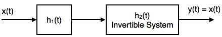
Y(S) = X(S) H1(S) H2(S)
= X(S) H1(S) $1 \over ( H1(S) )$ Since H2(S) = 1/( H1(S) )
$\therefore, $ Y(S) = X(S)
$\to$ y(t) = x(t)
Hence, the system is invertible.
If y(t) $\neq$ x(t), then the system is said to be non-invertible.
Stable and Unstable Systems
The system is said to be stable only when the output is bounded for bounded input. For a bounded input, if the output is unbounded in the system then it is said to be unstable.
Note: For a bounded signal, amplitude is finite.
Example 1: y (t) = x2(t)
Let the input is u(t) (unit step bounded input) then the output y(t) = u2(t) = u(t) = bounded output.
Hence, the system is stable.
Example 2: y (t) = $\int x(t)\, dt$
Let the input is u (t) (unit step bounded input) then the output y(t) = $\int u(t)\, dt$ = ramp signal (unbounded because amplitude of ramp is not finite it goes to infinite when t $\to$ infinite).
Hence, the system is unstable.
Signals Analysis
Analogy Between Vectors and Signals
There is a perfect analogy between vectors and signals.
Vector
A vector contains magnitude and direction. The name of the vector is denoted by bold face type and their magnitude is denoted by light face type.
Example: V is a vector with magnitude V. Consider two vectors V1 and V2 as shown in the following diagram. Let the component of V1 along with V2 is given by C12V2. The component of a vector V1 along with the vector V2 can obtained by taking a perpendicular from the end of V1 to the vector V2 as shown in diagram:

The vector V1 can be expressed in terms of vector V2
V1= C12V2 + Ve
Where Ve is the error vector.
But this is not the only way of expressing vector V1 in terms of V2. The alternate possibilities are:
V1=C1V2+Ve1

V2=C2V2+Ve2

The error signal is minimum for large component value. If C12=0, then two signals are said to be orthogonal.
Dot Product of Two Vectors
V1 . V2 = V1.V2 cosθ
θ = Angle between V1 and V2
V1 . V2 =V2.V1
The components of V1 alogn V2 = V1 Cos θ = $V1.V2 \over V2$
From the diagram, components of V1 alogn V2 = C 12 V2
$$V_1.V_2 \over V_2 = C_12\,V_2$$
$$ \Rightarrow C_{12} = {V_1.V_2 \over V_2}$$
Signal
The concept of orthogonality can be applied to signals. Let us consider two signals f1(t) and f2(t). Similar to vectors, you can approximate f1(t) in terms of f2(t) as
f1(t) = C12 f2(t) + fe(t) for (t1 < t < t2)
$ \Rightarrow $ fe(t) = f1(t) C12 f2(t)
One possible way of minimizing the error is integrating over the interval t1 to t2.
$${1 \over {t_2 - t_1}} \int_{t_1}^{t_2} [f_e (t)] dt$$
$${1 \over {t_2 - t_1}} \int_{t_1}^{t_2} [f_1(t) - C_{12}f_2(t)]dt $$
However, this step also does not reduce the error to appreciable extent. This can be corrected by taking the square of error function.
$\varepsilon = {1 \over {t_2 - t_1}} \int_{t_1}^{t_2} [f_e (t)]^2 dt$
$\Rightarrow {1 \over {t_2 - t_1}} \int_{t_1}^{t_2} [f_e (t) - C_{12}f_2]^2 dt $
Where ε is the mean square value of error signal. The value of C12 which minimizes the error, you need to calculate ${d\varepsilon \over dC_{12} } = 0 $
$\Rightarrow {d \over dC_{12} } [ {1 \over t_2 - t_1 } \int_{t_1}^{t_2} [f_1 (t) - C_{12} f_2 (t)]^2 dt]= 0 $
$\Rightarrow {1 \over {t_2 - t_1}} \int_{t_1}^{t_2} [ {d \over dC_{12} } f_{1}^2(t) - {d \over dC_{12} } 2f_1(t)C_{12}f_2(t)+ {d \over dC_{12} } f_{2}^{2} (t) C_{12}^2 ] dt =0 $
Derivative of the terms which do not have C12 term are zero.
$\Rightarrow \int_{t_1}^{t_2} - 2f_1(t) f_2(t) dt + 2C_{12}\int_{t_1}^{t_2}[f_{2}^{2} (t)]dt = 0 $
If $C_{12} = {{\int_{t_1}^{t_2}f_1(t)f_2(t)dt } \over {\int_{t_1}^{t_2} f_{2}^{2} (t)dt }} $ component is zero, then two signals are said to be orthogonal.
Put C12 = 0 to get condition for orthogonality.
0 = $ {{\int_{t_1}^{t_2}f_1(t)f_2(t)dt } \over {\int_{t_1}^{t_2} f_{2}^{2} (t)dt }} $
$$ \int_{t_1}^{t_2} f_1 (t)f_2(t) dt = 0 $$
Orthogonal Vector Space
A complete set of orthogonal vectors is referred to as orthogonal vector space. Consider a three dimensional vector space as shown below:
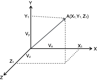
Consider a vector A at a point (X1, Y1, Z1). Consider three unit vectors (VX, VY, VZ) in the direction of X, Y, Z axis respectively. Since these unit vectors are mutually orthogonal, it satisfies that
$$V_X. V_X= V_Y. V_Y= V_Z. V_Z = 1 $$
$$V_X. V_Y= V_Y. V_Z= V_Z. V_X = 0 $$
You can write above conditions as
$$V_a . V_b = \left\{ \begin{array}{l l} 1 & \quad a = b \\ 0 & \quad a \neq b \end{array} \right. $$
The vector A can be represented in terms of its components and unit vectors as
$A = X_1 V_X + Y_1 V_Y + Z_1 V_Z................(1) $
Any vectors in this three dimensional space can be represented in terms of these three unit vectors only.
If you consider n dimensional space, then any vector A in that space can be represented as
$ A = X_1 V_X + Y_1 V_Y + Z_1 V_Z+...+ N_1V_N.....(2) $
As the magnitude of unit vectors is unity for any vector A
The component of A along x axis = A.VX
The component of A along Y axis = A.VY
The component of A along Z axis = A.VZ
Similarly, for n dimensional space, the component of A along some G axis
$= A.VG...............(3)$
Substitute equation 2 in equation 3.
$\Rightarrow CG= (X_1 V_X + Y_1 V_Y + Z_1 V_Z +...+G_1 V_G...+ N_1V_N)V_G$
$= X_1 V_X V_G + Y_1 V_Y V_G + Z_1 V_Z V_G +...+ G_1V_G V_G...+ N_1V_N V_G$
$= G_1 \,\,\,\,\, \text{since } V_G V_G=1$
$If V_G V_G \neq 1 \,\,\text{i.e.} V_G V_G= k$
$AV_G = G_1V_G V_G= G_1K$
$G_1 = {(AV_G) \over K}$
Orthogonal Signal Space
Let us consider a set of n mutually orthogonal functions x1(t), x2(t)... xn(t) over the interval t1 to t2. As these functions are orthogonal to each other, any two signals xj(t), xk(t) have to satisfy the orthogonality condition. i.e.
$$\int_{t_1}^{t_2} x_j(t)x_k(t)dt = 0 \,\,\, \text{where}\, j \neq k$$
$$\text{Let} \int_{t_1}^{t_2}x_{k}^{2}(t)dt = k_k $$
Let a function f(t), it can be approximated with this orthogonal signal space by adding the components along mutually orthogonal signals i.e.
$\,\,\,f(t) = C_1x_1(t) + C_2x_2(t) + ... + C_nx_n(t) + f_e(t) $
$\quad\quad=\Sigma_{r=1}^{n} C_rx_r (t) $
$\,\,\,f(t) = f(t) - \Sigma_{r=1}^n C_rx_r (t) $
Mean sqaure error $ \varepsilon = {1 \over t_2 - t_2 } \int_{t_1}^{t_2} [ f_e(t)]^2 dt$
$$ = {1 \over t_2 - t_2 } \int_{t_1}^{t_2} [ f[t] - \sum_{r=1}^{n} C_rx_r(t) ]^2 dt $$
The component which minimizes the mean square error can be found by
$$ {d\varepsilon \over dC_1} = {d\varepsilon \over dC_2} = ... = {d\varepsilon \over dC_k} = 0 $$
Let us consider ${d\varepsilon \over dC_k} = 0 $
$${d \over dC_k}[ {1 \over t_2 - t_1} \int_{t_1}^{t_2} [ f(t) - \Sigma_{r=1}^n C_rx_r(t)]^2 dt] = 0 $$
All terms that do not contain Ck is zero. i.e. in summation, r=k term remains and all other terms are zero.
$$\int_{t_1}^{t_2} - 2 f(t)x_k(t)dt + 2C_k \int_{t_1}^{t_2} [x_k^2 (t)] dt=0 $$
$$\Rightarrow C_k = {{\int_{t_1}^{t_2}f(t)x_k(t)dt} \over {int_{t_1}^{t_2} x_k^2 (t)dt}} $$
$$\Rightarrow \int_{t_1}^{t_2} f(t)x_k(t)dt = C_kK_k $$
Mean Square Error
The average of square of error function fe(t) is called as mean square error. It is denoted by ε (epsilon).
.$\varepsilon = {1 \over t_2 - t_1 } \int_{t_1}^{t_2} [f_e (t)]^2dt$
$\,\,\,\,= {1 \over t_2 - t_1 } \int_{t_1}^{t_2} [f_e (t) - \Sigma_{r=1}^n C_rx_r(t)]^2 dt $
$\,\,\,\,= {1 \over t_2 - t_1 } [ \int_{t_1}^{t_2} [f_e^2 (t) ]dt + \Sigma_{r=1}^{n} C_r^2 \int_{t_1}^{t_2} x_r^2 (t) dt - 2 \Sigma_{r=1}^{n} C_r \int_{t_1}^{t_2} x_r (t)f(t)dt$
You know that $C_{r}^{2} \int_{t_1}^{t_2} x_r^2 (t)dt = C_r \int_{t_1}^{t_2} x_r (t)f(d)dt = C_r^2 K_r $
$\varepsilon = {1 \over t_2 - t_1 } [ \int_{t_1}^{t_2} [f^2 (t)] dt + \Sigma_{r=1}^{n} C_r^2 K_r - 2 \Sigma_{r=1}^{n} C_r^2 K_r] $
$\,\,\,\,= {1 \over t_2 - t_1 } [\int_{t_1}^{t_2} [f^2 (t)] dt - \Sigma_{r=1}^{n} C_r^2 K_r ] $
$\, \therefore \varepsilon = {1 \over t_2 - t_1 } [\int_{t_1}^{t_2} [f^2 (t)] dt + (C_1^2 K_1 + C_2^2 K_2 + ... + C_n^2 K_n)] $
The above equation is used to evaluate the mean square error.
Closed and Complete Set of Orthogonal Functions
Let us consider a set of n mutually orthogonal functions x1(t), x2(t)...xn(t) over the interval t1 to t2. This is called as closed and complete set when there exist no function f(t) satisfying the condition $\int_{t_1}^{t_2} f(t)x_k(t)dt = 0 $
If this function is satisfying the equation $\int_{t_1}^{t_2} f(t)x_k(t)dt=0 \,\, \text{for}\, k = 1,2,..$ then f(t) is said to be orthogonal to each and every function of orthogonal set. This set is incomplete without f(t). It becomes closed and complete set when f(t) is included.
f(t) can be approximated with this orthogonal set by adding the components along mutually orthogonal signals i.e.
$$f(t) = C_1 x_1(t) + C_2 x_2(t) + ... + C_n x_n(t) + f_e(t) $$
If the infinite series $C_1 x_1(t) + C_2 x_2(t) + ... + C_n x_n(t)$ converges to f(t) then mean square error is zero.
Orthogonality in Complex Functions
If f1(t) and f2(t) are two complex functions, then f1(t) can be expressed in terms of f2(t) as
$f_1(t) = C_{12}f_2(t) \,\,\,\,\,\,\,\,$ ..with negligible error
Where $C_{12} = {{\int_{t_1}^{t_2} f_1(t)f_2^*(t)dt} \over { \int_{t_1}^{t_2} |f_2(t)|^2 dt}} $
Where $f_2^* (t)$ = complex conjugate of f2(t).
If f1(t) and f2(t) are orthogonal then C12 = 0
$$ {\int_{t_1}^{t_2} f_1 (t) f_2^*(t) dt \over \int_{t_1}^{t_2} |f_2 (t) |^2 dt} = 0 $$
$$\Rightarrow \int_{t_1}^{t_2} f_1 (t) f_2^* (dt) = 0$$
The above equation represents orthogonality condition in complex functions.
Fourier Series
Jean Baptiste Joseph Fourier,a French mathematician and a physicist; was born in Auxerre, France. He initialized Fourier series, Fourier transforms and their applications to problems of heat transfer and vibrations. The Fourier series, Fourier transforms and Fourier's Law are named in his honour.
Fourier series
To represent any periodic signal x(t), Fourier developed an expression called Fourier series. This is in terms of an infinite sum of sines and cosines or exponentials. Fourier series uses orthoganality condition.
Fourier Series Representation of Continuous Time Periodic Signals
A signal is said to be periodic if it satisfies the condition x (t) = x (t + T) or x (n) = x (n + N).
Where T = fundamental time period,
ω0= fundamental frequency = 2π/T
There are two basic periodic signals:
$x(t) = \cos\omega_0t$ (sinusoidal) &
$x(t) = e^{j\omega_0 t} $ (complex exponential)
These two signals are periodic with period $T= 2\pi/\omega_0$.
A set of harmonically related complex exponentials can be represented as {$\phi_k (t)$}
$${ \phi_k (t)} = \{ e^{jk\omega_0t}\} = \{ e^{jk({2\pi \over T})t}\} \text{where} \,k = 0 \pm 1, \pm 2 ..n \,\,\,.....(1) $$
All these signals are periodic with period T
According to orthogonal signal space approximation of a function x (t) with n, mutually orthogonal functions is given by
$$x(t) = \sum_{k = - \infty}^{\infty} a_k e^{jk\omega_0t} ..... (2) $$
$$ = \sum_{k = - \infty}^{\infty} a_kk e^{jk\omega_0t} $$
Where $a_k$= Fourier coefficient = coefficient of approximation.
This signal x(t) is also periodic with period T.
Equation 2 represents Fourier series representation of periodic signal x(t).
The term k = 0 is constant.
The term $k = \pm1$ having fundamental frequency $\omega_0$, is called as 1st harmonics.
The term $k = \pm2$ having fundamental frequency $2\omega_0$, is called as 2nd harmonics, and so on...
The term $k = n$ having fundamental frequency $n\omega0$, is called as nth harmonics.
Deriving Fourier Coefficient
We know that $x(t) = \Sigma_{k=- \infty}^{\infty} a_k e^{jk \omega_0 t} ...... (1)$
Multiply $e^{-jn\omega_0 t}$ on both sides. Then
$$ x(t)e^{-jn\omega_0 t} = \sum_{k=- \infty}^{\infty} a_k e^{jk \omega_0 t} . e^{-jn\omega_0 t} $$
Consider integral on both sides.
$$ \int_{0}^{T} x(t) e^{jk \omega_0 t} dt = \int_{0}^{T} \sum_{k=-\infty}^{\infty} a_k e^{jk \omega_0 t} . e^{-jn\omega_0 t}dt $$
$$ \quad \quad \quad \quad \,\, = \int_{0}^{T} \sum_{k=-\infty}^{\infty} a_k e^{j(k-n) \omega_0 t} . dt$$
$$ \int_{0}^{T} x(t) e^{jk \omega_0 t} dt = \sum_{k=-\infty}^{\infty} a_k \int_{0}^{T} e^{j(k-n) \omega_0 t} dt. \,\, ..... (2)$$
by Euler's formula,
$$ \int_{0}^{T} e^{j(k-n) \omega_0 t} dt. = \int_{0}^{T} \cos(k-n)\omega_0 dt + j \int_{0}^{T} \sin(k-n)\omega_0t\,dt$$
$$ \int_{0}^{T} e^{j(k-n) \omega_0 t} dt. = \left\{ \begin{array}{l l} T & \quad k = n \\ 0 & \quad k \neq n \end{array} \right. $$
Hence in equation 2, the integral is zero for all values of k except at k = n. Put k = n in equation 2.
$$\Rightarrow \int_{0}^{T} x(t) e^{-jn\omega_0 t} dt = a_n T $$
$$\Rightarrow a_n = {1 \over T} \int_{0}^{T} e^{-jn\omega_0 t} dt $$
Replace n by k.
$$\Rightarrow a_k = {1 \over T} \int_{0}^{T} e^{-jk\omega_0 t} dt$$
$$\therefore x(t) = \sum_{k=-\infty}^{\infty} a_k e^{j(k-n) \omega_0 t} $$
$$\text{where} a_k = {1 \over T} \int_{0}^{T} e^{-jk\omega_0 t} dt $$
Fourier Series Properties
These are properties of Fourier series:
Linearity Property
If $ x(t) \xleftarrow[\,]{fourier\,series}\xrightarrow[\,]{coefficient} f_{xn}$ & $ y(t) \xleftarrow[\,]{fourier\,series}\xrightarrow[\,]{coefficient} f_{yn}$
then linearity property states that
$ \text{a}\, x(t) + \text{b}\, y(t) \xleftarrow[\,]{fourier\,series}\xrightarrow[\,]{coefficient} \text{a}\, f_{xn} + \text{b}\, f_{yn}$
Time Shifting Property
If $ x(t) \xleftarrow[\,]{fourier\,series}\xrightarrow[\,]{coefficient} f_{xn}$
then time shifting property states that
$x(t-t_0) \xleftarrow[\,]{fourier\,series}\xrightarrow[\,]{coefficient} e^{-jn\omega_0 t_0}f_{xn} $
Frequency Shifting Property
If $ x(t) \xleftarrow[\,]{fourier\,series}\xrightarrow[\,]{coefficient} f_{xn}$
then frequency shifting property states that
$e^{jn\omega_0 t_0} . x(t) \xleftarrow[\,]{fourier\,series}\xrightarrow[\,]{coefficient} f_{x(n-n_0)} $
Time Reversal Property
If $ x(t) \xleftarrow[\,]{fourier\,series}\xrightarrow[\,]{coefficient} f_{xn}$
then time reversal property states that
If $ x(-t) \xleftarrow[\,]{fourier\,series}\xrightarrow[\,]{coefficient} f_{-xn}$
Time Scaling Property
If $ x(t) \xleftarrow[\,]{fourier\,series}\xrightarrow[\,]{coefficient} f_{xn}$
then time scaling property states that
If $ x(at) \xleftarrow[\,]{fourier\,series}\xrightarrow[\,]{coefficient} f_{xn}$
Time scaling property changes frequency components from $\omega_0$ to $a\omega_0$.
Differentiation and Integration Properties
If $ x(t) \xleftarrow[\,]{fourier\,series}\xrightarrow[\,]{coefficient} f_{xn}$
then differentiation property states that
If $ {dx(t)\over dt} \xleftarrow[\,]{fourier\,series}\xrightarrow[\,]{coefficient} jn\omega_0 . f_{xn}$
& integration property states that
If $ \int x(t) dt \xleftarrow[\,]{fourier\,series}\xrightarrow[\,]{coefficient} {f_{xn} \over jn\omega_0} $
Multiplication and Convolution Properties
If $ x(t) \xleftarrow[\,]{fourier\,series}\xrightarrow[\,]{coefficient} f_{xn}$ & $ y(t) \xleftarrow[\,]{fourier\,series}\xrightarrow[\,]{coefficient} f_{yn}$
then multiplication property states that
$ x(t) . y(t) \xleftarrow[\,]{fourier\,series}\xrightarrow[\,]{coefficient} T f_{xn} * f_{yn}$
& convolution property states that
$ x(t) * y(t) \xleftarrow[\,]{fourier\,series}\xrightarrow[\,]{coefficient} T f_{xn} . f_{yn}$
Conjugate and Conjugate Symmetry Properties
If $ x(t) \xleftarrow[\,]{fourier\,series}\xrightarrow[\,]{coefficient} f_{xn}$
Then conjugate property states that
$ x*(t) \xleftarrow[\,]{fourier\,series}\xrightarrow[\,]{coefficient} f*_{xn}$
Conjugate symmetry property for real valued time signal states that
$$f*_{xn} = f_{-xn}$$
& Conjugate symmetry property for imaginary valued time signal states that
$$f*_{xn} = -f_{-xn} $$
Fourier Series Types
Trigonometric Fourier Series (TFS)
$\sin n\omega_0 t$ and $\sin m\omega_0 t$ are orthogonal over the interval $(t_0, t_0+{2\pi \over \omega_0})$. So $\sin\omega_0 t,\, \sin 2\omega_0 t$ forms an orthogonal set. This set is not complete without {$\cos n\omega_0 t$ } because this cosine set is also orthogonal to sine set. So to complete this set we must include both cosine and sine terms. Now the complete orthogonal set contains all cosine and sine terms i.e. {$\sin n\omega_0 t,\,\cos n\omega_0 t$ } where n=0, 1, 2...
$\therefore$ Any function x(t) in the interval $(t_0, t_0+{2\pi \over \omega_0})$ can be represented as
$$ x(t) = a_0 \cos0\omega_0 t+ a_1 \cos 1\omega_0 t+ a_2 \cos2 \omega_0 t +...+ a_n \cos n\omega_0 t + ... $$
$$ + b_0 \sin 0\omega_0 t + b_1 \sin 1\omega_0 t +...+ b_n \sin n\omega_0 t + ... $$
$$ = a_0 + a_1 \cos 1\omega_0 t + a_2 \cos 2 \omega_0 t +...+ a_n \cos n\omega_0 t + ...$$
$$ + b_1 \sin 1\omega_0 t +...+ b_n \sin n\omega_0 t + ...$$
$$ \therefore x(t) = a_0 + \sum_{n=1}^{\infty} (a_n \cos n\omega_0 t + b_n \sin n\omega_0 t ) \quad (t_0< t < t_0+T)$$
The above equation represents trigonometric Fourier series representation of x(t).
$$\text{Where} \,a_0 = {\int_{t_0}^{t_0+T} x(t)1 dt \over \int_{t_0}^{t_0+T} 1^2 dt} = {1 \over T} \int_{t_0}^{t_0+T} x(t)dt $$
$$a_n = {\int_{t_0}^{t_0+T} x(t) \cos n\omega_0 t\,dt \over \int_{t_0}^{t_0+T} \cos ^2 n\omega_0 t\, dt}$$
$$b_n = {\int_{t_0}^{t_0+T} x(t) \sin n\omega_0 t\,dt \over \int_{t_0}^{t_0+T} \sin ^2 n\omega_0 t\, dt}$$
$$\text{Here}\, \int_{t_0}^{t_0+T} \cos ^2 n\omega_0 t\, dt = \int_{t_0}^{t_0+T} \sin ^2 n\omega_0 t\, dt = {T\over 2}$$
$$\therefore a_n = {2\over T} \int_{t_0}^{t_0+T} x(t) \cos n\omega_0 t\,dt$$
$$b_n = {2\over T} \int_{t_0}^{t_0+T} x(t) \sin n\omega_0 t\,dt$$
Exponential Fourier Series (EFS)
Consider a set of complex exponential functions $\left\{e^{jn\omega_0 t}\right\} (n=0, \pm1, \pm2...)$ which is orthogonal over the interval $(t_0, t_0+T)$. Where $T={2\pi \over \omega_0}$ . This is a complete set so it is possible to represent any function f(t) as shown below
$ f(t) = F_0 + F_1e^{j\omega_0 t} + F_2e^{j 2\omega_0 t} + ... + F_n e^{j n\omega_0 t} + ...$
$\quad \quad \,\,F_{-1}e^{-j\omega_0 t} + F_{-2}e^{-j 2\omega_0 t} +...+ F_{-n}e^{-j n\omega_0 t}+...$
$$ \therefore f(t) = \sum_{n=-\infty}^{\infty} F_n e^{j n\omega_0 t} \quad \quad (t_0< t < t_0+T) ....... (1) $$
Equation 1 represents exponential Fourier series representation of a signal f(t) over the interval (t0, t0+T). The Fourier coefficient is given as
$$ F_n = {\int_{t_0}^{t_0+T} f(t) (e^{j n\omega_0 t} )^* dt \over \int_{t_0}^{t_0+T} e^{j n\omega_0 t} (e^{j n\omega_0 t} )^* dt} $$
$$ \quad = {\int_{t_0}^{t_0+T} f(t) e^{-j n\omega_0 t} dt \over \int_{t_0}^{t_0+T} e^{-j n\omega_0 t} e^{j n\omega_0 t} dt} $$
$$ \quad \quad \quad \quad \quad \quad \quad \quad \quad \,\, = {\int_{t_0}^{t_0+T} f(t) e^{-j n\omega_0 t} dt \over \int_{t_0}^{t_0+T} 1\, dt} = {1 \over T} \int_{t_0}^{t_0+T} f(t) e^{-j n\omega_0 t} dt $$
$$ \therefore F_n = {1 \over T} \int_{t_0}^{t_0+T} f(t) e^{-j n\omega_0 t} dt $$
Relation Between Trigonometric and Exponential Fourier Series
Consider a periodic signal x(t), the TFS & EFS representations are given below respectively
$ x(t) = a_0 + \Sigma_{n=1}^{\infty}(a_n \cos n\omega_0 t + b_n \sin n\omega_0 t) ... ... (1)$
$ x(t) = \Sigma_{n=-\infty}^{\infty} F_n e^{j n\omega_0 t}$
$\quad \,\,\, = F_0 + F_1e^{j\omega_0 t} + F_2e^{j 2\omega_0 t} + ... + F_n e^{j n\omega_0 t} + ... $
$\quad \quad \quad \quad F_{-1} e^{-j\omega_0 t} + F_{-2}e^{-j 2\omega_0 t} + ... + F_{-n}e^{-j n\omega_0 t} + ... $
$ = F_0 + F_1(\cos \omega_0 t + j \sin\omega_0 t) + F_2(cos 2\omega_0 t + j \sin 2\omega_0 t) + ... + F_n(\cos n\omega_0 t+j \sin n\omega_0 t)+ ... + F_{-1}(\cos\omega_0 t-j \sin\omega_0 t) + F_{-2}(\cos 2\omega_0 t-j \sin 2\omega_0 t) + ... + F_{-n}(\cos n\omega_0 t-j \sin n\omega_0 t) + ... $
$ = F_0 + (F_1+ F_{-1}) \cos\omega_0 t + (F_2+ F_{-2}) \cos2\omega_0 t +...+ j(F_1 - F_{-1}) \sin\omega_0 t + j(F_2 - F_{-2}) \sin2\omega_0 t+... $
$ \therefore x(t) = F_0 + \Sigma_{n=1}^{\infty}( (F_n +F_{-n} ) \cos n\omega_0 t+j(F_n-F_{-n}) \sin n\omega_0 t) ... ... (2) $
Compare equation 1 and 2.
$a_0= F_0$
$a_n=F_n+F_{-n}$
$b_n = j(F_n-F_{-n} )$
Similarly,
$F_n = \frac12 (a_n - jb_n )$
$F_{-n} = \frac12 (a_n + jb_n )$
Fourier Transforms
The main drawback of Fourier series is, it is only applicable to periodic signals. There are some naturally produced signals such as nonperiodic or aperiodic, which we cannot represent using Fourier series. To overcome this shortcoming, Fourier developed a mathematical model to transform signals between time (or spatial) domain to frequency domain & vice versa, which is called 'Fourier transform'.
Fourier transform has many applications in physics and engineering such as analysis of LTI systems, RADAR, astronomy, signal processing etc.
Deriving Fourier transform from Fourier series
Consider a periodic signal f(t) with period T. The complex Fourier series representation of f(t) is given as
$$ f(t) = \sum_{k=-\infty}^{\infty} a_k e^{jk\omega_0 t} $$
$$ \quad \quad \quad \quad \quad = \sum_{k=-\infty}^{\infty} a_k e^{j {2\pi \over T_0} kt} ... ... (1) $$
Let ${1 \over T_0} = \Delta f$, then equation 1 becomes
$f(t) = \sum_{k=-\infty}^{\infty} a_k e^{j2\pi k \Delta ft} ... ... (2) $
but you know that
$a_k = {1\over T_0} \int_{t_0}^{t_0+T} f(t) e^{-j k\omega_0 t} dt$
Substitute in equation 2.
(2) $ \Rightarrow f(t) = \Sigma_{k=-\infty}^{\infty} {1 \over T_0} \int_{t_0}^{t_0+T} f(t) e^{-j k\omega_0 t} dt\, e^{j2\pi k \Delta ft} $
Let $t_0={T\over2}$
$ = \Sigma_{k=-\infty}^{\infty} [ \int_{-T\over2}^{T\over2} f(t) e^{-j2 \pi k \Delta ft} dt ] \, e^{j2 \pi k \Delta ft}.\Delta f $
In the limit as $T \to \infty, \Delta f$ approaches differential $df, k \Delta f$ becomes a continuous variable $f$, and summation becomes integration
$$ f(t) = lim_{T \to \infty} \left\{ \Sigma_{k=-\infty}^{\infty} [ \int_{-T\over2}^{T\over2} f(t) e^{-j2 \pi k \Delta ft} dt ] \, e^{j2 \pi k \Delta ft}.\Delta f \right\} $$
$$ = \int_{-\infty}^{\infty} [ \int_{-\infty}^{\infty}\,f(t) e^{-j2\pi ft} dt] e^{j2\pi ft} df $$
$$f(t) = \int_{-\infty}^{\infty}\, F[\omega] e^{j\omega t} d \omega$$
$\text{Where}\,F[\omega] = [ \int_{-\infty}^{\infty}\, f(t) e^{-j2 \pi ft} dt]$
Fourier transform of a signal $$f(t) = F[\omega] = [\int_{-\infty}^{\infty}\, f(t) e^{-j\omega t} dt]$$
Inverse Fourier Transform is $$f(t) = \int_{-\infty}^{\infty}\,F[\omega] e^{j\omega t} d \omega$$
Fourier Transform of Basic Functions
Let us go through Fourier Transform of basic functions:
FT of GATE Function

$$F[\omega] = AT Sa({\omega T \over 2})$$
FT of Impulse Function
$FT [\omega(t) ] = [\int_{- \infty}^{\infty} \delta (t) e^{-j\omega t} dt] $
$\quad \quad \quad \quad = e^{-j\omega t}\, |\, t = 0 $
$\quad \quad \quad \quad = e^{0} = 1 $
$\quad \therefore \delta (\omega) = 1 $
FT of Unit Step Function:
$U(\omega) = \pi \delta (\omega)+1/j\omega$
FT of Exponentials
$ e^{-at}u(t) \stackrel{\mathrm{F.T}}{\longleftrightarrow} 1/(a+j)$
$ e^{-at}u(t) \stackrel{\mathrm{F.T}}{\longleftrightarrow} 1/(a+j\omega )$
$ e^{-a\,|\,t\,|} \stackrel{\mathrm{F.T}}{\longleftrightarrow} {2a \over {a^2+^2}}$
$ e^{j \omega_0 t} \stackrel{\mathrm{F.T}}{\longleftrightarrow} \delta (\omega - \omega_0)$
FT of Signum Function
$ sgn(t) \stackrel{\mathrm{F.T}}{\longleftrightarrow} {2 \over j \omega }$
Conditions for Existence of Fourier Transform
Any function f(t) can be represented by using Fourier transform only when the function satisfies Dirichlets conditions. i.e.
The function f(t) has finite number of maxima and minima.
There must be finite number of discontinuities in the signal f(t),in the given interval of time.
It must be absolutely integrable in the given interval of time i.e.
$ \int_{-\infty}^{\infty}\, |\, f(t) | \, dt < \infty $
Discrete Time Fourier Transforms (DTFT)
The discrete-time Fourier transform (DTFT) or the Fourier transform of a discretetime sequence x[n] is a representation of the sequence in terms of the complex exponential sequence $e^{j\omega n}$.
The DTFT sequence x[n] is given by
$$ X(\omega) = \Sigma_{n= -\infty}^{\infty} x(n)e^{-j \omega n} \,\, ...\,... (1) $$
Here, X(ω) is a complex function of real frequency variable ω and it can be written as
$$ X(\omega) = X_{re}(\omega) + jX_{img}(\omega) $$
Where Xre(ω), Ximg(ω) are real and imaginary parts of X(ω) respectively.
$$ X_{re}(\omega) = |\, X(\omega) | \cos\theta(\omega) $$
$$ X_{img}(\omega) = |\, X(\omega) | \sin\theta(\omega) $$
$$ |X(\omega) |^2 = |\, X_{re} (\omega) |^2+ |\,X_{im} (\omega) |^2 $$
And X(ω) can also be represented as $ X(\omega) = |\,X(\omega) | e^{j\theta ()} $
Where $\theta(\omega) = arg{X(\omega) } $
$|\,X(\omega) |, \theta(\omega)$ are called magnitude and phase spectrums of X(ω).
Inverse Discrete-Time Fourier Transform
$$ x(n) = { 1 \over 2\pi} \int_{-\pi}^{\pi} X(\omega) e^{j \omega n} d\omega \,\, ...\,... (2)$$
Convergence Condition:
The infinite series in equation 1 may be converges or may not. x(n) is absolutely summable.
$$ \text{when}\,\, \sum_{n=-\infty}^{\infty} |\, x(n)|\, < \infty $$
An absolutely summable sequence has always a finite energy but a finite-energy sequence is not necessarily to be absolutely summable.
Fourier Transforms Properties
Here are the properties of Fourier Transform:
Linearity Property
$\text{If}\,\,x (t) \stackrel{\mathrm{F.T}}{\longleftrightarrow} X(\omega) $
$ \text{&} \,\, y(t) \stackrel{\mathrm{F.T}}{\longleftrightarrow} Y(\omega) $
Then linearity property states that
$a x (t) + b y (t) \stackrel{\mathrm{F.T}}{\longleftrightarrow} a X(\omega) + b Y(\omega) $
Time Shifting Property
$\text{If}\, x(t) \stackrel{\mathrm{F.T}}{\longleftrightarrow} X (\omega)$
Then Time shifting property states that
$x (t-t_0) \stackrel{\mathrm{F.T}}{\longleftrightarrow} e^{-j\omega t_0 } X(\omega)$
Frequency Shifting Property
$\text{If}\,\, x(t) \stackrel{\mathrm{F.T}}{\longleftrightarrow} X(\omega)$
Then frequency shifting property states that
$e^{j\omega_0 t} . x (t) \stackrel{\mathrm{F.T}}{\longleftrightarrow} X(\omega - \omega_0)$
Time Reversal Property
$ \text{If}\,\, x(t) \stackrel{\mathrm{F.T}}{\longleftrightarrow} X(\omega)$
Then Time reversal property states that
$ x (-t) \stackrel{\mathrm{F.T}}{\longleftrightarrow} X(-\omega)$
Time Scaling Property
$ \text{If}\,\, x (t) \stackrel{\mathrm{F.T}}{\longleftrightarrow} X(\omega) $
Then Time scaling property states that
$ x (at) {1 \over |\,a\,|} X { \omega \over a}$
Differentiation and Integration Properties
$ If \,\, x (t) \stackrel{\mathrm{F.T}}{\longleftrightarrow} X(\omega)$
Then Differentiation property states that
$ {dx (t) \over dt} \stackrel{\mathrm{F.T}}{\longleftrightarrow} j\omega . X(\omega)$
$ {d^n x (t) \over dt^n } \stackrel{\mathrm{F.T}}{\longleftrightarrow} (j \omega)^n . X(\omega) $
and integration property states that
$ \int x(t) \, dt \stackrel{\mathrm{F.T}}{\longleftrightarrow} {1 \over j \omega} X(\omega) $
$ \iiint ... \int x(t)\, dt \stackrel{\mathrm{F.T}}{\longleftrightarrow} { 1 \over (j\omega)^n} X(\omega) $
Multiplication and Convolution Properties
$ \text{If} \,\, x(t) \stackrel{\mathrm{F.T}}{\longleftrightarrow} X(\omega) $
$ \text{&} \,\,y(t) \stackrel{\mathrm{F.T}}{\longleftrightarrow} Y(\omega) $
Then multiplication property states that
$ x(t). y(t) \stackrel{\mathrm{F.T}}{\longleftrightarrow} X(\omega)*Y(\omega) $
and convolution property states that
$ x(t) * y(t) \stackrel{\mathrm{F.T}}{\longleftrightarrow} {1 \over 2 \pi} X(\omega).Y(\omega) $
Distortion Less Transmission
Transmission is said to be distortion-less if the input and output have identical wave shapes. i.e., in distortion-less transmission, the input x(t) and output y(t) satisfy the condition:
y (t) = Kx(t - td)
Where td = delay time and
k = constant.
Take Fourier transform on both sides
FT[ y (t)] = FT[Kx(t - td)]
= K FT[x(t - td)]
According to time shifting property,
= KX(w)$e^{-j \omega t_d}$
$ \therefore Y(w) = KX(w)e^{-j \omega t_d}$
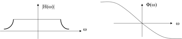
Thus, distortionless transmission of a signal x(t) through a system with impulse response h(t) is achieved when
$|H(\omega)| = K \,\, \text{and} \,\,\,\,$ (amplitude response)
$ \Phi (\omega) = -\omega t_d = -2\pi f t_d \,\,\, $ (phase response)
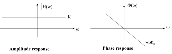
A physical transmission system may have amplitude and phase responses as shown below:
Hilbert Transform
Hilbert transform of a signal x(t) is defined as the transform in which phase angle of all components of the signal is shifted by $\pm \text{90}^o $.
Hilbert transform of x(t) is represented with $\hat{x}(t)$,and it is given by
$$ \hat{x}(t) = { 1 \over \pi } \int_{-\infty}^{\infty} {x(k) \over t-k } dk $$
The inverse Hilbert transform is given by
$$ \hat{x}(t) = { 1 \over \pi } \int_{-\infty}^{\infty} {x(k) \over t-k } dk $$
x(t), $\hat{x}$(t) is called a Hilbert transform pair.
Properties of the Hilbert Transform
A signal x(t) and its Hilbert transform $\hat{x}$(t) have
The same amplitude spectrum.
The same autocorrelation function.
The energy spectral density is same for both x(t) and $\hat{x}$(t).
x(t) and $\hat{x}$(t) are orthogonal.
The Hilbert transform of $\hat{x}$(t) is -x(t)
If Fourier transform exist then Hilbert transform also exists for energy and power signals.
Convolution and Correlation
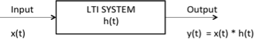
Convolution
Convolution is a mathematical operation used to express the relation between input and output of an LTI system. It relates input, output and impulse response of an LTI system as
$$ y (t) = x(t) * h(t) $$
Where y (t) = output of LTI
x (t) = input of LTI
h (t) = impulse response of LTI
There are two types of convolutions:
Continuous convolution
Discrete convolution
Continuous Convolution
$ y(t) \,\,= x (t) * h (t) $
$= \int_{-\infty}^{\infty} x(\tau) h (t-\tau)d\tau$
(or)
$= \int_{-\infty}^{\infty} x(t - \tau) h (\tau)d\tau $
Discrete Convolution
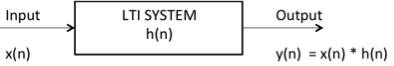
$y(n)\,\,= x (n) * h (n)$
$= \Sigma_{k = - \infty}^{\infty} x(k) h (n-k) $
(or)
$= \Sigma_{k = - \infty}^{\infty} x(n-k) h (k) $
By using convolution we can find zero state response of the system.
Deconvolution
Deconvolution is reverse process to convolution widely used in signal and image processing.
Properties of Convolution
Commutative Property
$ x_1 (t) * x_2 (t) = x_2 (t) * x_1 (t) $
Distributive Property
$ x_1 (t) * [x_2 (t) + x_3 (t) ] = [x_1 (t) * x_2 (t)] + [x_1 (t) * x_3 (t)]$
Associative Property
$x_1 (t) * [x_2 (t) * x_3 (t) ] = [x_1 (t) * x_2 (t)] * x_3 (t) $
Shifting Property
$ x_1 (t) * x_2 (t) = y (t) $
$ x_1 (t) * x_2 (t-t_0) = y (t-t_0) $
$ x_1 (t-t_0) * x_2 (t) = y (t-t_0) $
$ x_1 (t-t_0) * x_2 (t-t_1) = y (t-t_0-t_1) $
Convolution with Impulse
$ x_1 (t) * \delta (t) = x(t) $
$ x_1 (t) * \delta (t- t_0) = x(t-t_0) $
Convolution of Unit Steps
$ u (t) * u (t) = r(t) $
$ u (t-T_1) * u (t-T_2) = r(t-T_1-T_2) $
$ u (n) * u (n) = [n+1] u(n) $
Scaling Property
If $x (t) * h (t) = y (t) $
then $x (a t) * h (a t) = {1 \over |a|} y (a t)$
Differentiation of Output
if $y (t) = x (t) * h (t)$
then $ {dy (t) \over dt} = {dx(t) \over dt} * h (t) $
or
$ {dy (t) \over dt} = x (t) * {dh(t) \over dt}$
Note:
Convolution of two causal sequences is causal.
Convolution of two anti causal sequences is anti causal.
Convolution of two unequal length rectangles results a trapezium.
Convolution of two equal length rectangles results a triangle.
A function convoluted itself is equal to integration of that function.
Example: You know that $u(t) * u(t) = r(t)$
According to above note, $u(t) * u(t) = \int u(t)dt = \int 1dt = t = r(t)$
Here, you get the result just by integrating $u(t)$.
Limits of Convoluted Signal
If two signals are convoluted then the resulting convoluted signal has following range:
Sum of lower limits < t < sum of upper limits
Ex: find the range of convolution of signals given below

Here, we have two rectangles of unequal length to convolute, which results a trapezium.
The range of convoluted signal is:
Sum of lower limits < t < sum of upper limits
$-1+-2 < t < 2+2 $
$-3 < t < 4 $
Hence the result is trapezium with period 7.
Area of Convoluted Signal
The area under convoluted signal is given by $A_y = A_x A_h$
Where Ax = area under input signal
Ah = area under impulse response
Ay = area under output signal
Proof: $y(t) = \int_{-\infty}^{\infty} x(\tau) h (t-\tau)d\tau$
Take integration on both sides
$ \int y(t)dt \,\,\, =\int \int_{-\infty}^{\infty}\, x (\tau) h (t-\tau)d\tau dt $
$ =\int x (\tau) d\tau \int_{-\infty}^{\infty}\, h (t-\tau) dt $
We know that area of any signal is the integration of that signal itself.
$\therefore A_y = A_x\,A_h$
DC Component
DC component of any signal is given by
$\text{DC component}={\text{area of the signal} \over \text{period of the signal}}$
Ex: what is the dc component of the resultant convoluted signal given below?
Here area of x1(t) = length breadth = 1 3 = 3
area of x2(t) = length breadth = 1 4 = 4
area of convoluted signal = area of x1(t) area of x2(t)
= 3 4 = 12
Duration of the convoluted signal = sum of lower limits < t < sum of upper limits
= -1 + -2 < t < 2+2
= -3 < t < 4
Period=7
$\therefore$ Dc component of the convoluted signal = $\text{area of the signal} \over \text{period of the signal}$
Dc component = ${12 \over 7}$
Discrete Convolution
Let us see how to calculate discrete convolution:
i. To calculate discrete linear convolution:
Convolute two sequences x[n] = {a,b,c} & h[n] = [e,f,g]
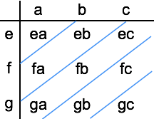
Convoluted output = [ ea, eb+fa, ec+fb+ga, fc+gb, gc]
Note: if any two sequences have m, n number of samples respectively, then the resulting convoluted sequence will have [m+n-1] samples.
Example: Convolute two sequences x[n] = {1,2,3} & h[n] = {-1,2,2}
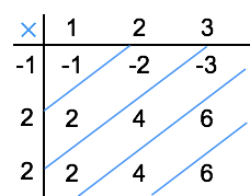
Convoluted output y[n] = [ -1, -2+2, -3+4+2, 6+4, 6]
= [-1, 0, 3, 10, 6]
Here x[n] contains 3 samples and h[n] is also having 3 samples so the resulting sequence having 3+3-1 = 5 samples.
ii. To calculate periodic or circular convolution:
Periodic convolution is valid for discrete Fourier transform. To calculate periodic convolution all the samples must be real. Periodic or circular convolution is also called as fast convolution.
If two sequences of length m, n respectively are convoluted using circular convolution then resulting sequence having max [m,n] samples.
Ex: convolute two sequences x[n] = {1,2,3} & h[n] = {-1,2,2} using circular convolution
Normal Convoluted output y[n] = [ -1, -2+2, -3+4+2, 6+4, 6].
= [-1, 0, 3, 10, 6]
Here x[n] contains 3 samples and h[n] also has 3 samples. Hence the resulting sequence obtained by circular convolution must have max[3,3]= 3 samples.
Now to get periodic convolution result, 1st 3 samples [as the period is 3] of normal convolution is same next two samples are added to 1st samples as shown below:

$\therefore$ Circular convolution result $y[n] = [9\quad 6\quad 3 ]$
Correlation
Correlation is a measure of similarity between two signals. The general formula for correlation is
$$ \int_{-\infty}^{\infty} x_1 (t)x_2 (t-\tau) dt $$
There are two types of correlation:
Auto correlation
Cros correlation
Auto Correlation Function
It is defined as correlation of a signal with itself. Auto correlation function is a measure of similarity between a signal & its time delayed version. It is represented with R($\tau$).
Consider a signals x(t). The auto correlation function of x(t) with its time delayed version is given by
$$ R_{11} (\tau) = R (\tau) = \int_{-\infty}^{\infty} x(t)x(t-\tau) dt \quad \quad \text{[+ve shift]} $$
$$\quad \quad \quad \quad \quad = \int_{-\infty}^{\infty} x(t)x(t + \tau) dt \quad \quad \text{[-ve shift]} $$
Where $\tau$ = searching or scanning or delay parameter.
If the signal is complex then auto correlation function is given by
$$ R_{11} (\tau) = R (\tau) = \int_{-\infty}^{\infty} x(t)x * (t-\tau) dt \quad \quad \text{[+ve shift]} $$
$$\quad \quad \quad \quad \quad = \int_{-\infty}^{\infty} x(t + \tau)x * (t) dt \quad \quad \text{[-ve shift]} $$
Properties of Auto-correlation Function of Energy Signal
Auto correlation exhibits conjugate symmetry i.e. R ($\tau$) = R*(-$\tau$)
Auto correlation function of energy signal at origin i.e. at $\tau$=0 is equal to total energy of that signal, which is given as:
R (0) = E = $ \int_{-\infty}^{\infty}\,|\,x(t)\,|^2\,dt $
Auto correlation function $\infty {1 \over \tau} $,
Auto correlation function is maximum at $\tau$=0 i.e |R ($\tau$) | ≤ R (0) ∀ $\tau$
Auto correlation function and energy spectral densities are Fourier transform pairs. i.e.
$F.T\,[ R (\tau) ] = \Psi(\omega)$
$\Psi(\omega) = \int_{-\infty}^{\infty} R (\tau) e^{-j\omega \tau} d \tau$
$ R (\tau) = x (\tau)* x(-\tau) $
Auto Correlation Function of Power Signals
The auto correlation function of periodic power signal with period T is given by
$$ R (\tau) = \lim_{T \to \infty} {1\over T} \int_{{-T \over 2}}^{{T \over 2}}\, x(t) x* (t-\tau) dt $$
Properties
Auto correlation of power signal exhibits conjugate symmetry i.e. $ R (\tau) = R*(-\tau)$
Auto correlation function of power signal at $\tau = 0$ (at origin)is equal to total power of that signal. i.e.
$R (0)= \rho $
Auto correlation function of power signal $\infty {1 \over \tau}$,
Auto correlation function of power signal is maximum at $\tau$ = 0 i.e.,
$ | R (\tau) | \leq R (0)\, \forall \,\tau$
Auto correlation function and power spectral densities are Fourier transform pairs. i.e.,
$F.T[ R (\tau) ] = s(\omega)$
$s(\omega) = \int_{-\infty}^{\infty} R (\tau) e^{-j\omega \tau} d\tau$
$R (\tau) = x (\tau)* x(-\tau) $
Density Spectrum
Let us see density spectrums:
Energy Density Spectrum
Energy density spectrum can be calculated using the formula:
$$ E = \int_{-\infty}^{\infty} |\,x(f)\,|^2 df $$
Power Density Spectrum
Power density spectrum can be calculated by using the formula:
$$P = \Sigma_{n = -\infty}^{\infty}\, |\,C_n |^2 $$
Cross Correlation Function
Cross correlation is the measure of similarity between two different signals.
Consider two signals x1(t) and x2(t). The cross correlation of these two signals $R_{12}(\tau)$ is given by
$$R_{12} (\tau) = \int_{-\infty}^{\infty} x_1 (t)x_2 (t-\tau)\, dt \quad \quad \text{[+ve shift]} $$
$$\quad \quad = \int_{-\infty}^{\infty} x_1 (t+\tau)x_2 (t)\, dt \quad \quad \text{[-ve shift]}$$
If signals are complex then
$$R_{12} (\tau) = \int_{-\infty}^{\infty} x_1 (t)x_2^{*}(t-\tau)\, dt \quad \quad \text{[+ve shift]} $$
$$\quad \quad = \int_{-\infty}^{\infty} x_1 (t+\tau)x_2^{*} (t)\, dt \quad \quad \text{[-ve shift]}$$
$$R_{21} (\tau) = \int_{-\infty}^{\infty} x_2 (t)x_1^{*}(t-\tau)\, dt \quad \quad \text{[+ve shift]} $$
$$\quad \quad = \int_{-\infty}^{\infty} x_2 (t+\tau)x_1^{*} (t)\, dt \quad \quad \text{[-ve shift]}$$
Properties of Cross Correlation Function of Energy and Power Signals
Auto correlation exhibits conjugate symmetry i.e. $R_{12} (\tau) = R^*_{21} (-\tau)$.
Cross correlation is not commutative like convolution i.e.
$$ R_{12} (\tau) \neq R_{21} (-\tau) $$
-
If R12(0) = 0 means, if $ \int_{-\infty}^{\infty} x_1 (t) x_2^* (t) dt = 0$, then the two signals are said to be orthogonal.
For power signal if $ \lim_{T \to \infty} {1\over T} \int_{{-T \over 2}}^{{T \over 2}}\, x(t) x^* (t)\,dt $ then two signals are said to be orthogonal.
Cross correlation function corresponds to the multiplication of spectrums of one signal to the complex conjugate of spectrum of another signal. i.e.
$$ R_{12} (\tau) \leftarrow \rightarrow X_1(\omega) X_2^*(\omega)$$
This also called as correlation theorem.
Parseval's Theorem
Parseval's theorem for energy signals states that the total energy in a signal can be obtained by the spectrum of the signal as
$ E = {1\over 2 \pi} \int_{-\infty}^{\infty} |X(\omega)|^2 d\omega $
Note: If a signal has energy E then time scaled version of that signal x(at) has energy E/a.
Signals Sampling Theorem
Statement: A continuous time signal can be represented in its samples and can be recovered back when sampling frequency fs is greater than or equal to the twice the highest frequency component of message signal. i. e.
$$ f_s \geq 2 f_m. $$
Proof: Consider a continuous time signal x(t). The spectrum of x(t) is a band limited to fm Hz i.e. the spectrum of x(t) is zero for |ω|>ωm.
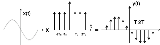
Sampling of input signal x(t) can be obtained by multiplying x(t) with an impulse train δ(t) of period Ts. The output of multiplier is a discrete signal called sampled signal which is represented with y(t) in the following diagrams:
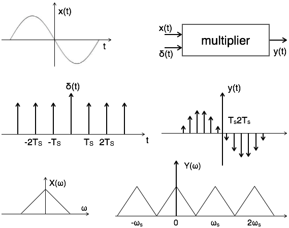
Here, you can observe that the sampled signal takes the period of impulse. The process of sampling can be explained by the following mathematical expression:
$ \text{Sampled signal}\, y(t) = x(t) . \delta(t) \,\,...\,...(1) $
The trigonometric Fourier series representation of $\delta$(t) is given by
$ \delta(t)= a_0 + \Sigma_{n=1}^{\infty}(a_n \cos n\omega_s t + b_n \sin n\omega_s t )\,\,...\,...(2) $
Where $ a_0 = {1\over T_s} \int_{-T \over 2}^{ T \over 2} \delta (t)dt = {1\over T_s} \delta(0) = {1\over T_s} $
$ a_n = {2 \over T_s} \int_{-T \over 2}^{T \over 2} \delta (t) \cos n\omega_s\, dt = { 2 \over T_2} \delta (0) \cos n \omega_s 0 = {2 \over T}$
$b_n = {2 \over T_s} \int_{-T \over 2}^{T \over 2} \delta(t) \sin n\omega_s t\, dt = {2 \over T_s} \delta(0) \sin n\omega_s 0 = 0 $
Substitute above values in equation 2.
$\therefore\, \delta(t)= {1 \over T_s} + \Sigma_{n=1}^{\infty} ( { 2 \over T_s} \cos n\omega_s t+0)$
Substitute δ(t) in equation 1.
$\to y(t) = x(t) . \delta(t) $
$ = x(t) [{1 \over T_s} + \Sigma_{n=1}^{\infty}({2 \over T_s} \cos n\omega_s t) ] $
$ = {1 \over T_s} [x(t) + 2 \Sigma_{n=1}^{\infty} (\cos n\omega_s t) x(t) ] $
$ y(t) = {1 \over T_s} [x(t) + 2\cos \omega_s t.x(t) + 2 \cos 2\omega_st.x(t) + 2 \cos 3\omega_s t.x(t) \,...\, ...\,] $
Take Fourier transform on both sides.
$Y(\omega) = {1 \over T_s} [X(\omega)+X(\omega-\omega_s )+X(\omega+\omega_s )+X(\omega-2\omega_s )+X(\omega+2\omega_s )+ \,...] $
$\therefore\,\, Y(\omega) = {1\over T_s} \Sigma_{n=-\infty}^{\infty} X(\omega - n\omega_s )\quad\quad where \,\,n= 0,\pm1,\pm2,... $
To reconstruct x(t), you must recover input signal spectrum X(ω) from sampled signal spectrum Y(ω), which is possible when there is no overlapping between the cycles of Y(ω).
Possibility of sampled frequency spectrum with different conditions is given by the following diagrams:

Aliasing Effect
The overlapped region in case of under sampling represents aliasing effect, which can be removed by
considering fs >2fm
By using anti aliasing filters.
Signals Sampling Techniques
There are three types of sampling techniques:
Impulse sampling.
Natural sampling.
Flat Top sampling.
Impulse Sampling
Impulse sampling can be performed by multiplying input signal x(t) with impulse train $\Sigma_{n=-\infty}^{\infty}\delta(t-nT)$ of period 'T'. Here, the amplitude of impulse changes with respect to amplitude of input signal x(t). The output of sampler is given by
$y(t) = x(t) $ impulse train
$= x(t) \Sigma_{n=-\infty}^{\infty} \delta(t-nT)$
$ y(t) = y_{\delta} (t) = \Sigma_{n=-\infty}^{\infty}x(nt) \delta(t-nT)\,...\,... 1 $
To get the spectrum of sampled signal, consider Fourier transform of equation 1 on both sides
$Y(\omega) = {1 \over T} \Sigma_{n=-\infty}^{\infty} X(\omega - n \omega_s ) $
This is called ideal sampling or impulse sampling. You cannot use this practically because pulse width cannot be zero and the generation of impulse train is not possible practically.
Natural Sampling
Natural sampling is similar to impulse sampling, except the impulse train is replaced by pulse train of period T. i.e. you multiply input signal x(t) to pulse train $\Sigma_{n=-\infty}^{\infty} P(t-nT)$ as shown below
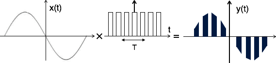
The output of sampler is
$y(t) = x(t) \times \text{pulse train}$
$= x(t) \times p(t) $
$= x(t) \times \Sigma_{n=-\infty}^{\infty} P(t-nT)\,...\,...(1) $
The exponential Fourier series representation of p(t) can be given as
$p(t) = \Sigma_{n=-\infty}^{\infty} F_n e^{j n\omega_s t}\,...\,...(2) $
$= \Sigma_{n=-\infty}^{\infty} F_n e^{j 2 \pi nf_s t} $
Where $F_n= {1 \over T} \int_{-T \over 2}^{T \over 2} p(t) e^{-j n \omega_s t} dt$
$= {1 \over TP}(n \omega_s)$
Substitute Fn value in equation 2
$ \therefore p(t) = \Sigma_{n=-\infty}^{\infty} {1 \over T} P(n \omega_s)e^{j n \omega_s t}$
$ = {1 \over T} \Sigma_{n=-\infty}^{\infty} P(n \omega_s)e^{j n \omega_s t}$
Substitute p(t) in equation 1
$y(t) = x(t) \times p(t)$
$= x(t) \times {1 \over T} \Sigma_{n=-\infty}^{\infty} P(n \omega_s)\,e^{j n \omega_s t} $
$y(t) = {1 \over T} \Sigma_{n=-\infty}^{\infty} P( n \omega_s)\, x(t)\, e^{j n \omega_s t} $
To get the spectrum of sampled signal, consider the Fourier transform on both sides.
$F.T\, [ y(t)] = F.T [{1 \over T} \Sigma_{n=-\infty}^{\infty} P( n \omega_s)\, x(t)\, e^{j n \omega_s t}]$
$ = {1 \over T} \Sigma_{n=-\infty}^{\infty} P( n \omega_s)\,F.T\,[ x(t)\, e^{j n \omega_s t} ] $
According to frequency shifting property
$F.T\,[ x(t)\, e^{j n \omega_s t} ] = X[\omega-n\omega_s] $
$ \therefore\, Y[\omega] = {1 \over T} \Sigma_{n=-\infty}^{\infty} P( n \omega_s)\,X[\omega-n\omega_s] $
Flat Top Sampling
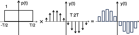
During transmission, noise is introduced at top of the transmission pulse which can be easily removed if the pulse is in the form of flat top. Here, the top of the samples are flat i.e. they have constant amplitude. Hence, it is called as flat top sampling or practical sampling. Flat top sampling makes use of sample and hold circuit.
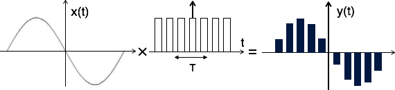
Theoretically, the sampled signal can be obtained by convolution of rectangular pulse p(t) with ideally sampled signal say yδ(t) as shown in the diagram:
i.e. $ y(t) = p(t) \times y_\delta (t)\, ... \, ...(1) $
To get the sampled spectrum, consider Fourier transform on both sides for equation 1
$Y[\omega] = F.T\,[P(t) \times y_\delta (t)] $
By the knowledge of convolution property,
$Y[\omega] = P(\omega)\, Y_\delta (\omega)$
Here $P(\omega) = T Sa({\omega T \over 2}) = 2 \sin \omega T/ \omega$
Nyquist Rate
It is the minimum sampling rate at which signal can be converted into samples and can be recovered back without distortion.
Nyquist rate fN = 2fm hz
Nyquist interval = ${1 \over fN}$ = $ {1 \over 2fm}$ seconds.
Samplings of Band Pass Signals
In case of band pass signals, the spectrum of band pass signal X[ω] = 0 for the frequencies outside the range f1 ≤ f ≤ f2. The frequency f1 is always greater than zero. Plus, there is no aliasing effect when fs > 2f2. But it has two disadvantages:
The sampling rate is large in proportion with f2. This has practical limitations.
The sampled signal spectrum has spectral gaps.
To overcome this, the band pass theorem states that the input signal x(t) can be converted into its samples and can be recovered back without distortion when sampling frequency fs < 2f2.
Also,
$$ f_s = {1 \over T} = {2f_2 \over m} $$
Where m is the largest integer < ${f_2 \over B}$
and B is the bandwidth of the signal. If f2=KB, then
$$ f_s = {1 \over T} = {2KB \over m} $$
For band pass signals of bandwidth 2fm and the minimum sampling rate fs= 2 B = 4fm,
the spectrum of sampled signal is given by $Y[\omega] = {1 \over T} \Sigma_{n=-\infty}^{\infty}\,X[ \omega - 2nB]$
Laplace Transforms (LT)
Complex Fourier transform is also called as Bilateral Laplace Transform. This is used to solve differential equations. Consider an LTI system exited by a complex exponential signal of the form x(t) = Gest.
Where s = any complex number = $\sigma + j\omega$,
σ = real of s, and
ω = imaginary of s
The response of LTI can be obtained by the convolution of input with its impulse response i.e.
$ y(t) = x(t) \times h(t) = \int_{-\infty}^{\infty}\, h (\tau)\, x (t-\tau)d\tau $
$= \int_{-\infty}^{\infty}\, h (\tau)\, Ge^{s(t-\tau)}d\tau $
$= Ge^{st}. \int_{-\infty}^{\infty}\, h (\tau)\, e^{(-s \tau)}d\tau $
$ y(t) = Ge^{st}.H(S) = x(t).H(S)$
Where H(S) = Laplace transform of $h(\tau) = \int_{-\infty}^{\infty} h (\tau) e^{-s\tau} d\tau $
Similarly, Laplace transform of $x(t) = X(S) = \int_{-\infty}^{\infty} x(t) e^{-st} dt\,...\,...(1)$
Relation between Laplace and Fourier transforms
Laplace transform of $x(t) = X(S) =\int_{-\infty}^{\infty} x(t) e^{-st} dt$
Substitute s= σ + jω in above equation.
$ X(\sigma+j\omega) =\int_{-\infty}^{\infty}\,x (t) e^{-(\sigma+j\omega)t} dt$
$ = \int_{-\infty}^{\infty} [ x (t) e^{-\sigma t}] e^{-j\omega t} dt $
$\therefore X(S) = F.T [x (t) e^{-\sigma t}]\,...\,...(2)$
$X(S) = X(\omega) \quad\quad for\,\, s= j\omega$
Inverse Laplace Transform
You know that $X(S) = F.T [x (t) e^{-\sigma t}]$
$\to x (t) e^{-\sigma t} = F.T^{-1} [X(S)] = F.T^{-1} [X(\sigma+j\omega)]$
$= {1\over 2}\pi \int_{-\infty}^{\infty} X(\sigma+j\omega) e^{j\omega t} d\omega$
$ x (t) = e^{\sigma t} {1 \over 2\pi} \int_{-\infty}^{\infty} X(\sigma+j\omega) e^{j\omega t} d\omega $
$= {1 \over 2\pi} \int_{-\infty}^{\infty} X(\sigma+j\omega) e^{(\sigma+j\omega)t} d\omega \,...\,...(3)$
Here, $\sigma+j\omega = s$
$jd = ds d = ds/j$
$ \therefore x (t) = {1 \over 2\pi j} \int_{-\infty}^{\infty} X(s) e^{st} ds\,...\,...(4) $
Equations 1 and 4 represent Laplace and Inverse Laplace Transform of a signal x(t).
Conditions for Existence of Laplace Transform
Dirichlet's conditions are used to define the existence of Laplace transform. i.e.
The function f(t) has finite number of maxima and minima.
There must be finite number of discontinuities in the signal f(t),in the given interval of time.
It must be absolutely integrable in the given interval of time. i.e.
$ \int_{-\infty}^{\infty} |\,f(t)|\, dt \lt \infty $
Initial and Final Value Theorems
If the Laplace transform of an unknown function x(t) is known, then it is possible to determine the initial and the final values of that unknown signal i.e. x(t) at t=0+ and t=∞.
Initial Value Theorem
Statement: if x(t) and its 1st derivative is Laplace transformable, then the initial value of x(t) is given by
$$ x(0^+) = \lim_{s \to \infty} SX(S) $$
Final Value Theorem
Statement: if x(t) and its 1st derivative is Laplace transformable, then the final value of x(t) is given by
$$ x(\infty) = \lim_{s \to \infty} SX(S) $$
Laplace Transforms Properties
The properties of Laplace transform are:
Linearity Property
If $\,x (t) \stackrel{\mathrm{L.T}}{\longleftrightarrow} X(s)$
& $\, y(t) \stackrel{\mathrm{L.T}}{\longleftrightarrow} Y(s)$
Then linearity property states that
$a x (t) + b y (t) \stackrel{\mathrm{L.T}}{\longleftrightarrow} a X(s) + b Y(s)$
Time Shifting Property
If $\,x (t) \stackrel{\mathrm{L.T}}{\longleftrightarrow} X(s)$
Then time shifting property states that
$x (t-t_0) \stackrel{\mathrm{L.T}}{\longleftrightarrow} e^{-st_0 } X(s)$
Frequency Shifting Property
If $\, x (t) \stackrel{\mathrm{L.T}}{\longleftrightarrow} X(s)$
Then frequency shifting property states that
$e^{s_0 t} . x (t) \stackrel{\mathrm{L.T}}{\longleftrightarrow} X(s-s_0)$
Time Reversal Property
If $\,x (t) \stackrel{\mathrm{L.T}}{\longleftrightarrow} X(s)$
Then time reversal property states that
$x (-t) \stackrel{\mathrm{L.T}}{\longleftrightarrow} X(-s)$
Time Scaling Property
If $\,x (t) \stackrel{\mathrm{L.T}}{\longleftrightarrow} X(s)$
Then time scaling property states that
$x (at) \stackrel{\mathrm{L.T}}{\longleftrightarrow} {1\over |a|} X({s\over a})$
Differentiation and Integration Properties
If $\, x (t) \stackrel{\mathrm{L.T}}{\longleftrightarrow} X(s)$
Then differentiation property states that
$ {dx (t) \over dt} \stackrel{\mathrm{L.T}}{\longleftrightarrow} s. X(s) - s. X(0) $
${d^n x (t) \over dt^n} \stackrel{\mathrm{L.T}}{\longleftrightarrow} (s)^n . X(s)$
The integration property states that
$\int x (t) dt \stackrel{\mathrm{L.T}}{\longleftrightarrow} {1 \over s} X(s)$
$\iiint \,...\, \int x (t) dt \stackrel{\mathrm{L.T}}{\longleftrightarrow} {1 \over s^n} X(s)$
Multiplication and Convolution Properties
If $\,x(t) \stackrel{\mathrm{L.T}}{\longleftrightarrow} X(s)$
and $ y(t) \stackrel{\mathrm{L.T}}{\longleftrightarrow} Y(s)$
Then multiplication property states that
$x(t). y(t) \stackrel{\mathrm{L.T}}{\longleftrightarrow} {1 \over 2 \pi j} X(s)*Y(s)$
The convolution property states that
$x(t) * y(t) \stackrel{\mathrm{L.T}}{\longleftrightarrow} X(s).Y(s)$
Region of Convergence (ROC)
The range variation of for which the Laplace transform converges is called region of convergence.
Properties of ROC of Laplace Transform
ROC contains strip lines parallel to jω axis in s-plane.

If x(t) is absolutely integral and it is of finite duration, then ROC is entire s-plane.
If x(t) is a right sided sequence then ROC : Re{s} > σo.
If x(t) is a left sided sequence then ROC : Re{s} < σo.
If x(t) is a two sided sequence then ROC is the combination of two regions.
ROC can be explained by making use of examples given below:
Example 1: Find the Laplace transform and ROC of $x(t) = e-^{at}u(t)$
$L.T[x(t)] = L.T[e-^{at}u(t)] = {1 \over S+a}$
$ Re{} \gt -a $
$ ROC:Re{s} \gt >-a$

Example 2: Find the Laplace transform and ROC of $x(t) = e^{at}u(-t)$
$ L.T[x(t)] = L.T[e^{at}u(t)] = {1 \over S-a} $
$ Re{s} < a $
$ ROC: Re{s} < a $

Example 3: Find the Laplace transform and ROC of $x(t) = e^{-at}u(t)+e^{at}u(-t)$
$L.T[x(t)] = L.T[e^{-at}u(t)+e^{at}u(-t)] = {1 \over S+a} + {1 \over S-a}$
For ${1 \over S+a} Re\{s\} \gt -a $
For ${1 \over S-a} Re\{s\} \lt a $

Referring to the above diagram, combination region lies from a to a. Hence,
$ ROC: -a < Re{s} < a $
Causality and Stability
For a system to be causal, all poles of its transfer function must be right half of s-plane.

A system is said to be stable when all poles of its transfer function lay on the left half of s-plane.

A system is said to be unstable when at least one pole of its transfer function is shifted to the right half of s-plane.

A system is said to be marginally stable when at least one pole of its transfer function lies on the jω axis of s-plane.

ROC of Basic Functions
| f(t) | F(s) | ROC |
|---|---|---|
| $u(t)$ | $${1\over s}$$ | ROC: Re{s} > 0 |
| $ t\, u(t) $ | $${1\over s^2} $$ | ROC:Re{s} > 0 |
| $ t^n\, u(t) $ | $$ {n! \over s^{n+1}} $$ | ROC:Re{s} > 0 |
| $ e^{at}\, u(t) $ | $$ {1\over s-a} $$ | ROC:Re{s} > a |
| $ e^{-at}\, u(t) $ | $$ {1\over s+a} $$ | ROC:Re{s} > -a |
| $ e^{at}\, u(t) $ | $$ - {1\over s-a} $$ | ROC:Re{s} < a |
| $ e^{-at}\, u(-t) $ | $$ - {1\over s+a} $$ | ROC:Re{s} < -a |
| $ t\, e^{at}\, u(t) $ | $$ {1 \over (s-a)^2} $$ | ROC:Re{s} > a |
| $ t^{n} e^{at}\, u(t) $ | $$ {n! \over (s-a)^{n+1}} $$ | ROC:Re{s} > a |
| $ t\, e^{-at}\, u(t) $ | $$ {1 \over (s+a)^2} $$ | ROC:Re{s} > -a |
| $ t^n\, e^{-at}\, u(t) $ | $${n! \over (s+a)^{n+1}} $$ | ROC:Re{s} > -a |
| $ t\, e^{at}\, u(-t) $ | $$ - {1 \over (s-a)^2} $$ | ROC:Re{s} < a |
| $ t^n\, e^{at}\, u(-t) $ | $$ - {n! \over (s-a)^{n+1}} $$ | ROC:Re{s} < a |
| $ t\, e^{-at}\,u(-t) $ | $$ - {1 \over (s+a)^2} $$ | ROC:Re{s} < -a |
| $ t^n\, e^{-at}\, u(-t) $ | $$ - {n! \over (s+a)^{n+1}} $$ | ROC:Re{s} < -a |
| $ e^{-at} \cos \, bt $ | $$ {s+a \over (s+a)^2 + b^2 } $$ | |
| $ e^{-at} \sin\, bt $ | $$ {b \over (s+a)^2 + b^2 } $$ |
Z-Transforms (ZT)
Analysis of continuous time LTI systems can be done using z-transforms. It is a powerful mathematical tool to convert differential equations into algebraic equations.
The bilateral (two sided) z-transform of a discrete time signal x(n) is given as
$Z.T[x(n)] = X(Z) = \Sigma_{n = -\infty}^{\infty} x(n)z^{-n} $
The unilateral (one sided) z-transform of a discrete time signal x(n) is given as
$Z.T[x(n)] = X(Z) = \Sigma_{n = 0}^{\infty} x(n)z^{-n} $
Z-transform may exist for some signals for which Discrete Time Fourier Transform (DTFT) does not exist.
Concept of Z-Transform and Inverse Z-Transform
Z-transform of a discrete time signal x(n) can be represented with X(Z), and it is defined as
$X(Z) = \Sigma_{n=- \infty }^ {\infty} x(n)z^{-n} \,...\,...\,(1)$
If $Z = re^{j\omega}$ then equation 1 becomes
$X(re^{j\omega}) = \Sigma_{n=- \infty}^{\infty} x(n)[re^{j \omega} ]^{-n}$
$= \Sigma_{n=- \infty}^{\infty} x(n)[r^{-n} ] e^{-j \omega n}$
$X(re^{j \omega} ) = X(Z) = F.T[x(n)r^{-n}] \,...\,...\,(2) $
The above equation represents the relation between Fourier transform and Z-transform.
$ X(Z) |_{z=e^{j \omega}} = F.T [x(n)]. $
Inverse Z-transform
$X(re^{j \omega}) = F.T[x(n)r^{-n}] $
$x(n)r^{-n} = F.T^{-1}[X(re^{j \omega}]$
$x(n) = r^n\,F.T^{-1}[X(re^{j \omega} )]$
$= r^n {1 \over 2\pi} \int X(re{^j \omega} )e^{j \omega n} d \omega $
$= {1 \over 2\pi} \int X(re{^j \omega} )[re^{j \omega} ]^n d \omega \,...\,...\,(3)$
Substitute $re^{j \omega} = z$.
$dz = jre^{j \omega} d \omega = jz d \omega$
$d \omega = {1 \over j }z^{-1}dz$
Substitute in equation 3.
$ 3\, \to \, x(n) = {1 \over 2\pi} \int\, X(z)z^n {1 \over j } z^{-1} dz = {1 \over 2\pi j} \int \,X(z) z^{n-1} dz $
$$X(Z) = \sum_{n=- \infty }^{\infty} \,x(n)z^{-n}$$ $$x(n) = {1 \over 2\pi j} \int\, X(z) z^{n-1} dz$$
Z-Transforms Properties
Z-Transform has following properties:
Linearity Property
If $\,x (n) \stackrel{\mathrm{Z.T}}{\longleftrightarrow} X(Z)$
and $\,y(n) \stackrel{\mathrm{Z.T}}{\longleftrightarrow} Y(Z)$
Then linearity property states that
$a\, x (n) + b\, y (n) \stackrel{\mathrm{Z.T}}{\longleftrightarrow} a\, X(Z) + b\, Y(Z)$
Time Shifting Property
If $\,x (n) \stackrel{\mathrm{Z.T}}{\longleftrightarrow} X(Z)$
Then Time shifting property states that
$x (n-m) \stackrel{\mathrm{Z.T}}{\longleftrightarrow} z^{-m} X(Z)$
Multiplication by Exponential Sequence Property
If $\,x (n) \stackrel{\mathrm{Z.T}}{\longleftrightarrow} X(Z)$
Then multiplication by an exponential sequence property states that
$a^n\, . x(n) \stackrel{\mathrm{Z.T}}{\longleftrightarrow} X(Z/a)$
Time Reversal Property
If $\, x (n) \stackrel{\mathrm{Z.T}}{\longleftrightarrow} X(Z)$
Then time reversal property states that
$x (-n) \stackrel{\mathrm{Z.T}}{\longleftrightarrow} X(1/Z)$
Differentiation in Z-Domain OR Multiplication by n Property
If $\, x (n) \stackrel{\mathrm{Z.T}}{\longleftrightarrow} X(Z)$
Then multiplication by n or differentiation in z-domain property states that
$ n^k x (n) \stackrel{\mathrm{Z.T}}{\longleftrightarrow} [-1]^k z^k{d^k X(Z) \over dZ^K} $
Convolution Property
If $\,x (n) \stackrel{\mathrm{Z.T}}{\longleftrightarrow} X(Z)$
and $\,y(n) \stackrel{\mathrm{Z.T}}{\longleftrightarrow} Y(Z)$
Then convolution property states that
$x(n) * y(n) \stackrel{\mathrm{Z.T}}{\longleftrightarrow} X(Z).Y(Z)$
Correlation Property
If $\,x (n) \stackrel{\mathrm{Z.T}}{\longleftrightarrow} X(Z)$
and $\,y(n) \stackrel{\mathrm{Z.T}}{\longleftrightarrow} Y(Z)$
Then correlation property states that
$x(n) \otimes y(n) \stackrel{\mathrm{Z.T}}{\longleftrightarrow} X(Z).Y(Z^{-1})$
Initial Value and Final Value Theorems
Initial value and final value theorems of z-transform are defined for causal signal.
Initial Value Theorem
For a causal signal x(n), the initial value theorem states that
$ x (0) = \lim_{z \to \infty }X(z) $
This is used to find the initial value of the signal without taking inverse z-transform
Final Value Theorem
For a causal signal x(n), the final value theorem states that
$ x ( \infty ) = \lim_{z \to 1} [z-1] X(z) $
This is used to find the final value of the signal without taking inverse z-transform.
Region of Convergence (ROC) of Z-Transform
The range of variation of z for which z-transform converges is called region of convergence of z-transform.
Properties of ROC of Z-Transforms
ROC of z-transform is indicated with circle in z-plane.
ROC does not contain any poles.
If x(n) is a finite duration causal sequence or right sided sequence, then the ROC is entire z-plane except at z = 0.
If x(n) is a finite duration anti-causal sequence or left sided sequence, then the ROC is entire z-plane except at z = ∞.
If x(n) is a infinite duration causal sequence, ROC is exterior of the circle with radius a. i.e. |z| > a.
If x(n) is a infinite duration anti-causal sequence, ROC is interior of the circle with radius a. i.e. |z| < a.
If x(n) is a finite duration two sided sequence, then the ROC is entire z-plane except at z = 0 & z = ∞.
The concept of ROC can be explained by the following example:
Example 1: Find z-transform and ROC of $a^n u[n] + a^{-}nu[-n-1]$
$Z.T[a^n u[n]] + Z.T[a^{-n}u[-n-1]] = {Z \over Z-a} + {Z \over Z {-1 \over a}}$
$$ ROC: |z| \gt a \quad\quad ROC: |z| \lt {1 \over a} $$
The plot of ROC has two conditions as a > 1 and a < 1, as you do not know a.
In this case, there is no combination ROC.
Here, the combination of ROC is from $a \lt |z| \lt {1 \over a}$
Hence for this problem, z-transform is possible when a < 1.
Causality and Stability
Causality condition for discrete time LTI systems is as follows:
A discrete time LTI system is causal when
ROC is outside the outermost pole.
In The transfer function H[Z], the order of numerator cannot be grater than the order of denominator.
Stability Condition for Discrete Time LTI Systems
A discrete time LTI system is stable when
its system function H[Z] include unit circle |z|=1.
all poles of the transfer function lay inside the unit circle |z|=1.
Z-Transform of Basic Signals
| x(t) | X[Z] |
|---|---|
| $\delta$ | 1 |
| $u(n)$ | ${Z\over Z-1}$ |
| $u(-n-1)$ | $ -{Z\over Z-1}$ |
| $\delta(n-m)$ | $z^{-m}$ |
| $a^n u[n]$ | ${Z \over Z-a}$ |
| $a^n u[-n-1]$ | $- {Z \over Z-a}$ |
| $n\,a^n u[n]$ | ${aZ \over |Z-a|^2}$ |
| $n\,a^n u[-n-1] $ | $- {aZ \over |Z-a|^2}$ |
| $a^n \cos \omega n u[n] $ | ${Z^2-aZ \cos \omega \over Z^2-2aZ \cos \omega +a^2}$ |
| $a^n \sin \omega n u[n] $ | $ {aZ \sin \omega \over Z^2 -2aZ \cos \omega +a^2 } $ |
