Signals and Systems – Time Scaling of Signals

What is Time Scaling?

The process of multiplying a constant to the time axis of a signal is known as time scaling of the signal. The time scaling of signal may be time compression or time expansion depending upon the value of the constant or scaling factor. The time scaling operation of signals is very useful when data is to be fed at some rate and is to be taken out at a different rate.

Time scaling of continuous-time signal

The time scaling of a continuous time signal x(t) can be accomplished by replacing ‘t’ by ‘𝛼t’ in the function. Mathematically, it is given by,

𝑥(𝑡) → 𝑦(𝑡) = 𝑥(𝛼𝑡)

Where, α is a constant, called the scaling factor.

If α > 1, then the signal is compressed in time by a factor α and the time scaling of the signal is called the time compression. Whereas, if α < 1, then the signal is expanded in time by the factor α and the time scaling is said to be time expansion.

Example

Consider a continuous-time signal x(t) as shown in Figure-1. As it can be seen that the signal x(t) is increasing linearly from 0 to 5 in the time interval t = (-2) to t = 0 and remaining constant at 5 in the time interval t = 0 to t = 3 and then decreasing linearly from 5 to 0 in the time interval t = 3 to t = 5.

Case I – Consider the time scaling (compression) of the signal as,

𝑥(𝑡) → 𝑦(𝑡) = 𝑥(2𝑡)

As the value of scaling factor α = 2, i.e., α > 1, thus there is the time compression of the signal and the compressed signal is shown in Figure-2.

Here, it can be seen that the time compressed signal x(2t) increases linearly from 0 to 5 in the time interval 𝑡 = − (2/2) to 𝑡 = 0 and remains constant at 5 in the time interval t = 0 to t = (3/2) and then decreases linearly from 5 to 0 in the time interval t = (3/2) to t = (5/2).

Case II – Consider the time scaling (expansion) of the signal as,

$$\mathrm{x(t)\rightarrow y(t)=x\left ( \frac{t}{2} \right )}$$

In this case, the value of α = (1/2), i.e., α < 1, hence there is the time expansion of the signal as shown in Figure-3.

In Figure-3, the time expanded signal x(t/2) increases linearly from 0 to 5 in the time interval t = (-2×2) to t = 0, remains constant at 5 in the interval t = 0 to t = (3×2) and then decreases linearly from 5 to 0 in the interval t = (3×2) to t = (5×2).

Time Scaling of Discrete-Time Sequence

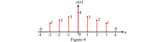
Consider a discrete time sequence x(n) as shown in Figure-4.

The time scaling for the discrete sequence can be defined as,

𝑥(𝑛) → 𝑦(𝑛) = 𝑥(𝑘𝑛)

Case I – If k = 2, then

𝑥(𝑛) → 𝑦(𝑛) = 𝑥(2𝑛)

Here, k > 1, thus the signal is compressed in time. We can plot the time compressed signal y(n) by substituting different values of n as shown in Figure-5.

𝑛 = 0 → 𝑦(0) = 𝑥(0) = 1

𝑛 = (−1) → 𝑦(−1) = 𝑥(−2) = −2

𝑛 = (−2) → 𝑦(−2) = 𝑥(−4) = 0

𝑛 = 1 → 𝑦(1) = 𝑥(2) = 2

𝑛 = 2 → 𝑦(2) = 𝑥(4) = 0

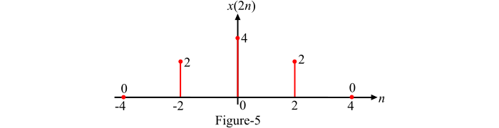
Therefore, to plot the signal x(2n), we have to skip the odd numbered samples in the signal x(n).

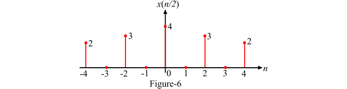
Case II – If k = (1/2), then

$$\mathrm{x(n)\rightarrow y(n)=x\left ( \frac{n}{2} \right )}$$

Since k < 1, hence the signal is expanded by a factor 2. We can plot the time expanded signal y(n) by substituting different values of n as follows −

𝑛 = 0 → 𝑦(0) = 𝑥(0) = 1

𝑛 = 2 → 𝑦(2) = 𝑥(1) = 3

𝑛 = 4 → 𝑦(4) = 𝑥(2) = 2

𝑛 = (−2) → 𝑦(−2) = 𝑥(−1) = 3

𝑛 = (−4) → 𝑦(−4) = 𝑥(−2) = 2

In this case, all odd components in x(n/2) are zero because the signal x(n) does not have any value in between the sampling instants. Figure-6 shows the plot of the signal $\mathrm{y(n)=x\left ( \frac{n}{2} \right )}$

Manish Kumar Saini

Updated on: 12-Nov-2021

12K+ Views

Kickstart Your Career

Get certified by completing the course

Get Started