- Signals & Systems Home
- Signals & Systems Overview
- Introduction
- Signals Basic Types
- Signals Classification
- Signals Basic Operations
- Systems Classification
- Types of Signals
- Representation of a Discrete Time Signal
- Continuous-Time Vs Discrete-Time Sinusoidal Signal
- Even and Odd Signals
- Properties of Even and Odd Signals
- Periodic and Aperiodic Signals
- Unit Step Signal
- Unit Ramp Signal
- Unit Parabolic Signal
- Energy Spectral Density
- Unit Impulse Signal
- Power Spectral Density
- Properties of Discrete Time Unit Impulse Signal
- Real and Complex Exponential Signals
- Addition and Subtraction of Signals
- Amplitude Scaling of Signals
- Multiplication of Signals
- Time Scaling of Signals
- Time Shifting Operation on Signals
- Time Reversal Operation on Signals
- Even and Odd Components of a Signal
- Energy and Power Signals
- Power of an Energy Signal over Infinite Time
- Energy of a Power Signal over Infinite Time
- Causal, Non-Causal, and Anti-Causal Signals
- Rectangular, Triangular, Signum, Sinc, and Gaussian Functions
- Signals Analysis
- Types of Systems
- What is a Linear System?
- Time Variant and Time-Invariant Systems
- Linear and Non-Linear Systems
- Static and Dynamic System
- Causal and Non-Causal System
- Stable and Unstable System
- Invertible and Non-Invertible Systems
- Linear Time-Invariant Systems
- Transfer Function of LTI System
- Properties of LTI Systems
- Response of LTI System
- Fourier Series
- Fourier Series
- Fourier Series Representation of Periodic Signals
- Fourier Series Types
- Trigonometric Fourier Series Coefficients
- Exponential Fourier Series Coefficients
- Complex Exponential Fourier Series
- Relation between Trigonometric & Exponential Fourier Series
- Fourier Series Properties
- Properties of Continuous-Time Fourier Series
- Time Differentiation and Integration Properties of Continuous-Time Fourier Series
- Time Shifting, Time Reversal, and Time Scaling Properties of Continuous-Time Fourier Series
- Linearity and Conjugation Property of Continuous-Time Fourier Series
- Multiplication or Modulation Property of Continuous-Time Fourier Series
- Convolution Property of Continuous-Time Fourier Series
- Convolution Property of Fourier Transform
- Parseval’s Theorem in Continuous Time Fourier Series
- Average Power Calculations of Periodic Functions Using Fourier Series
- GIBBS Phenomenon for Fourier Series
- Fourier Cosine Series
- Trigonometric Fourier Series
- Derivation of Fourier Transform from Fourier Series
- Difference between Fourier Series and Fourier Transform
- Wave Symmetry
- Even Symmetry
- Odd Symmetry
- Half Wave Symmetry
- Quarter Wave Symmetry
- Fourier Transform
- Fourier Transforms
- Fourier Transforms Properties
- Fourier Transform – Representation and Condition for Existence
- Properties of Continuous-Time Fourier Transform
- Table of Fourier Transform Pairs
- Linearity and Frequency Shifting Property of Fourier Transform
- Modulation Property of Fourier Transform
- Time-Shifting Property of Fourier Transform
- Time-Reversal Property of Fourier Transform
- Time Scaling Property of Fourier Transform
- Time Differentiation Property of Fourier Transform
- Time Integration Property of Fourier Transform
- Frequency Derivative Property of Fourier Transform
- Parseval’s Theorem & Parseval’s Identity of Fourier Transform
- Fourier Transform of Complex and Real Functions
- Fourier Transform of a Gaussian Signal
- Fourier Transform of a Triangular Pulse
- Fourier Transform of Rectangular Function
- Fourier Transform of Signum Function
- Fourier Transform of Unit Impulse Function
- Fourier Transform of Unit Step Function
- Fourier Transform of Single-Sided Real Exponential Functions
- Fourier Transform of Two-Sided Real Exponential Functions
- Fourier Transform of the Sine and Cosine Functions
- Fourier Transform of Periodic Signals
- Conjugation and Autocorrelation Property of Fourier Transform
- Duality Property of Fourier Transform
- Analysis of LTI System with Fourier Transform
- Relation between Discrete-Time Fourier Transform and Z Transform
- Convolution and Correlation
- Convolution in Signals and Systems
- Convolution and Correlation
- Correlation in Signals and Systems
- System Bandwidth vs Signal Bandwidth
- Time Convolution Theorem
- Frequency Convolution Theorem
- Energy Spectral Density and Autocorrelation Function
- Autocorrelation Function of a Signal
- Cross Correlation Function and its Properties
- Detection of Periodic Signals in the Presence of Noise (by Autocorrelation)
- Detection of Periodic Signals in the Presence of Noise (by Cross-Correlation)
- Autocorrelation Function and its Properties
- PSD and Autocorrelation Function
- Sampling
- Signals Sampling Theorem
- Nyquist Rate and Nyquist Interval
- Signals Sampling Techniques
- Effects of Undersampling (Aliasing) and Anti Aliasing Filter
- Different Types of Sampling Techniques
- Laplace Transform
- Laplace Transforms
- Common Laplace Transform Pairs
- Laplace Transform of Unit Impulse Function and Unit Step Function
- Laplace Transform of Sine and Cosine Functions
- Laplace Transform of Real Exponential and Complex Exponential Functions
- Laplace Transform of Ramp Function and Parabolic Function
- Laplace Transform of Damped Sine and Cosine Functions
- Laplace Transform of Damped Hyperbolic Sine and Cosine Functions
- Laplace Transform of Periodic Functions
- Laplace Transform of Rectifier Function
- Laplace Transforms Properties
- Linearity Property of Laplace Transform
- Time Shifting Property of Laplace Transform
- Time Scaling and Frequency Shifting Properties of Laplace Transform
- Time Differentiation Property of Laplace Transform
- Time Integration Property of Laplace Transform
- Time Convolution and Multiplication Properties of Laplace Transform
- Initial Value Theorem of Laplace Transform
- Final Value Theorem of Laplace Transform
- Parseval's Theorem for Laplace Transform
- Laplace Transform and Region of Convergence for right sided and left sided signals
- Laplace Transform and Region of Convergence of Two Sided and Finite Duration Signals
- Circuit Analysis with Laplace Transform
- Step Response and Impulse Response of Series RL Circuit using Laplace Transform
- Step Response and Impulse Response of Series RC Circuit using Laplace Transform
- Step Response of Series RLC Circuit using Laplace Transform
- Solving Differential Equations with Laplace Transform
- Difference between Laplace Transform and Fourier Transform
- Difference between Z Transform and Laplace Transform
- Relation between Laplace Transform and Z-Transform
- Relation between Laplace Transform and Fourier Transform
- Laplace Transform – Time Reversal, Conjugation, and Conjugate Symmetry Properties
- Laplace Transform – Differentiation in s Domain
- Laplace Transform – Conditions for Existence, Region of Convergence, Merits & Demerits
- Z Transform
- Z-Transforms (ZT)
- Common Z-Transform Pairs
- Z-Transform of Unit Impulse, Unit Step, and Unit Ramp Functions
- Z-Transform of Sine and Cosine Signals
- Z-Transform of Exponential Functions
- Z-Transforms Properties
- Properties of ROC of the Z-Transform
- Z-Transform and ROC of Finite Duration Sequences
- Conjugation and Accumulation Properties of Z-Transform
- Time Shifting Property of Z Transform
- Time Reversal Property of Z Transform
- Time Expansion Property of Z Transform
- Differentiation in z Domain Property of Z Transform
- Initial Value Theorem of Z-Transform
- Final Value Theorem of Z Transform
- Solution of Difference Equations Using Z Transform
- Long Division Method to Find Inverse Z Transform
- Partial Fraction Expansion Method for Inverse Z-Transform
- What is Inverse Z Transform?
- Inverse Z-Transform by Convolution Method
- Transform Analysis of LTI Systems using Z-Transform
- Convolution Property of Z Transform
- Correlation Property of Z Transform
- Multiplication by Exponential Sequence Property of Z Transform
- Multiplication Property of Z Transform
- Residue Method to Calculate Inverse Z Transform
- System Realization
- Cascade Form Realization of Continuous-Time Systems
- Direct Form-I Realization of Continuous-Time Systems
- Direct Form-II Realization of Continuous-Time Systems
- Parallel Form Realization of Continuous-Time Systems
- Causality and Paley Wiener Criterion for Physical Realization
- Discrete Fourier Transform
- Discrete-Time Fourier Transform
- Properties of Discrete Time Fourier Transform
- Linearity, Periodicity, and Symmetry Properties of Discrete-Time Fourier Transform
- Time Shifting and Frequency Shifting Properties of Discrete Time Fourier Transform
- Inverse Discrete-Time Fourier Transform
- Time Convolution and Frequency Convolution Properties of Discrete-Time Fourier Transform
- Differentiation in Frequency Domain Property of Discrete Time Fourier Transform
- Parseval’s Power Theorem
- Miscellaneous Concepts
- What is Mean Square Error?
- What is Fourier Spectrum?
- Region of Convergence
- Hilbert Transform
- Properties of Hilbert Transform
- Symmetric Impulse Response of Linear-Phase System
- Filter Characteristics of Linear Systems
- Characteristics of an Ideal Filter (LPF, HPF, BPF, and BRF)
- Zero Order Hold and its Transfer Function
- What is Ideal Reconstruction Filter?
- What is the Frequency Response of Discrete Time Systems?
- Basic Elements to Construct the Block Diagram of Continuous Time Systems
- BIBO Stability Criterion
- BIBO Stability of Discrete-Time Systems
- Distortion Less Transmission
- Distortionless Transmission through a System
- Rayleigh’s Energy Theorem
Laplace Transform and Region of Convergence of Two-Sided and Finite Duration Signals
What is Region of Convergence?
Region of Convergence (ROC) is defined as the set of points in s-plane for which the Laplace transform of a function $\mathrm{x\left ( t \right )}$ converges. In other words, the range of Re(s) (i.e., σ) for which the function X(s) converges is called the region of convergence.
ROC of Two-Sided Signals
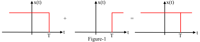
A signal $\mathrm{x\left ( t \right )}$ is said to be a two sided signal if it extends from -∞ to +∞. The two sided signal can be represented as the sum of two non-overlapping signals, one of which is right-sided signal and the other is the left-sided signal as shown in Figure- 1.
For a two-sided signal, the ROC of the Laplace transform X(s) is in the form of a strip in the s-plane bounded by two lines σ = σr and σ = σi.
Numerical Example - 1
Find the Laplace transform and ROC of the two-sided signal $\mathrm{x(t)\:=\:2e^{-3t}\:u(t)\:+\:3e^{4t}\:u(-t)}$
Solution
The given signal is,
$$\mathrm{x(t) \:=\: 2e^{-3t}\:u(t)\:+\:3e^{4t}\:u(-t)}$$
As the given signal is a two sided signal. The Laplace transform of signal x(t) is given by,
$$\mathrm{L[x(t)] \:=\: 2L\left [e^{-3t}\:u(t)\right ]\:+\:3L\left [e^{4t}\:u(-t) \right]}$$
$$\mathrm{\Rightarrow\:X(s)\:=\:\frac{2}{s\:+\:3}\:-\:\frac{3}{s-4}\:;\:ROC\:\to\:Re(s)\:\gt\:-3\:and\:Re(s)\:\lt\: 4}$$
Therefore, the ROC of the Laplace transform of the signal $\mathrm{x(t)}$ is,
$$\mathrm{Re(s)\:\gt\:-3\:\cap\:Re(s)\:\lt\:4\:=\:-3\:\lt\:Re(s)\:\lt\:4}$$

The ROC of the Laplace transform of the given signal x(t) is shown in Figure- 2. It can be seen that the ROC of the given two sided signal is a strip in the s-plane and lies to the right of the pole at s = −3 and to the left of the pole at s = +4.
ROC of Finite Duration Signals
A signal $\mathrm{x(t)}$ is said to be a finite duration signal if $\mathrm{x(t) \:=\: 0}$ for $\mathrm{t\:lt\:T_{1}}$ and $\mathrm{t\:gt\:T_{2}}$ where $\mathrm{T_{1}}$ and $\mathrm{T_{2}}$ are some finite time instants as shown in Figure-3.
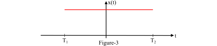
For a finite duration signal which is absolutely integrable, the ROC of its Laplace transform extends over the entire s-plane.
Numerical Example 2
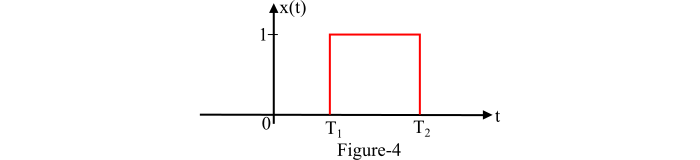
Find the Laplace transform and ROC of the finite duration signal $\mathrm{x(t)}$ shown in Figure-4.
Solution
The equation describing the given finite duration signal is given by,
$$\mathrm{x(t)\:=\:\left[ u(t\:-\:T_{1})\:-\:u(t\:-\:T_{2}) \right]}$$
Both the terms of this signal are causal. The Laplace transform of this is signal is obtained as −
$$\mathrm{L[x(t)]\:=\:L\left [u(t\:-\:T_{1})\right]\:-\:L\left [u(t\:-\:T_{2}) \right]}$$
$$\mathrm{\Rightarrow\: X(s)\:=\:\left (\frac{e^{-T_{1}s}}{s}\:-\:\frac{e^{-T_{2}s}}{s} \right )}$$
$$\mathrm{\therefore\: X(s)\:=\:\frac{1}{s}\left ({e^{-T_{1}s}}\:-\:{e^{-T_{2}s}} \right)\:;\: ROC\:\rightarrow\: All\: s}$$