- Signals & Systems Home
- Signals & Systems Overview
- Introduction
- Signals Basic Types
- Signals Classification
- Signals Basic Operations
- Systems Classification
- Types of Signals
- Representation of a Discrete Time Signal
- Continuous-Time Vs Discrete-Time Sinusoidal Signal
- Even and Odd Signals
- Properties of Even and Odd Signals
- Periodic and Aperiodic Signals
- Unit Step Signal
- Unit Ramp Signal
- Unit Parabolic Signal
- Energy Spectral Density
- Unit Impulse Signal
- Power Spectral Density
- Properties of Discrete Time Unit Impulse Signal
- Real and Complex Exponential Signals
- Addition and Subtraction of Signals
- Amplitude Scaling of Signals
- Multiplication of Signals
- Time Scaling of Signals
- Time Shifting Operation on Signals
- Time Reversal Operation on Signals
- Even and Odd Components of a Signal
- Energy and Power Signals
- Power of an Energy Signal over Infinite Time
- Energy of a Power Signal over Infinite Time
- Causal, Non-Causal, and Anti-Causal Signals
- Rectangular, Triangular, Signum, Sinc, and Gaussian Functions
- Signals Analysis
- Types of Systems
- What is a Linear System?
- Time Variant and Time-Invariant Systems
- Linear and Non-Linear Systems
- Static and Dynamic System
- Causal and Non-Causal System
- Stable and Unstable System
- Invertible and Non-Invertible Systems
- Linear Time-Invariant Systems
- Transfer Function of LTI System
- Properties of LTI Systems
- Response of LTI System
- Fourier Series
- Fourier Series
- Fourier Series Representation of Periodic Signals
- Fourier Series Types
- Trigonometric Fourier Series Coefficients
- Exponential Fourier Series Coefficients
- Complex Exponential Fourier Series
- Relation between Trigonometric & Exponential Fourier Series
- Fourier Series Properties
- Properties of Continuous-Time Fourier Series
- Time Differentiation and Integration Properties of Continuous-Time Fourier Series
- Time Shifting, Time Reversal, and Time Scaling Properties of Continuous-Time Fourier Series
- Linearity and Conjugation Property of Continuous-Time Fourier Series
- Multiplication or Modulation Property of Continuous-Time Fourier Series
- Convolution Property of Continuous-Time Fourier Series
- Convolution Property of Fourier Transform
- Parseval’s Theorem in Continuous Time Fourier Series
- Average Power Calculations of Periodic Functions Using Fourier Series
- GIBBS Phenomenon for Fourier Series
- Fourier Cosine Series
- Trigonometric Fourier Series
- Derivation of Fourier Transform from Fourier Series
- Difference between Fourier Series and Fourier Transform
- Wave Symmetry
- Even Symmetry
- Odd Symmetry
- Half Wave Symmetry
- Quarter Wave Symmetry
- Fourier Transform
- Fourier Transforms
- Fourier Transforms Properties
- Fourier Transform – Representation and Condition for Existence
- Properties of Continuous-Time Fourier Transform
- Table of Fourier Transform Pairs
- Linearity and Frequency Shifting Property of Fourier Transform
- Modulation Property of Fourier Transform
- Time-Shifting Property of Fourier Transform
- Time-Reversal Property of Fourier Transform
- Time Scaling Property of Fourier Transform
- Time Differentiation Property of Fourier Transform
- Time Integration Property of Fourier Transform
- Frequency Derivative Property of Fourier Transform
- Parseval’s Theorem & Parseval’s Identity of Fourier Transform
- Fourier Transform of Complex and Real Functions
- Fourier Transform of a Gaussian Signal
- Fourier Transform of a Triangular Pulse
- Fourier Transform of Rectangular Function
- Fourier Transform of Signum Function
- Fourier Transform of Unit Impulse Function
- Fourier Transform of Unit Step Function
- Fourier Transform of Single-Sided Real Exponential Functions
- Fourier Transform of Two-Sided Real Exponential Functions
- Fourier Transform of the Sine and Cosine Functions
- Fourier Transform of Periodic Signals
- Conjugation and Autocorrelation Property of Fourier Transform
- Duality Property of Fourier Transform
- Analysis of LTI System with Fourier Transform
- Relation between Discrete-Time Fourier Transform and Z Transform
- Convolution and Correlation
- Convolution in Signals and Systems
- Convolution and Correlation
- Correlation in Signals and Systems
- System Bandwidth vs Signal Bandwidth
- Time Convolution Theorem
- Frequency Convolution Theorem
- Energy Spectral Density and Autocorrelation Function
- Autocorrelation Function of a Signal
- Cross Correlation Function and its Properties
- Detection of Periodic Signals in the Presence of Noise (by Autocorrelation)
- Detection of Periodic Signals in the Presence of Noise (by Cross-Correlation)
- Autocorrelation Function and its Properties
- PSD and Autocorrelation Function
- Sampling
- Signals Sampling Theorem
- Nyquist Rate and Nyquist Interval
- Signals Sampling Techniques
- Effects of Undersampling (Aliasing) and Anti Aliasing Filter
- Different Types of Sampling Techniques
- Laplace Transform
- Laplace Transforms
- Common Laplace Transform Pairs
- Laplace Transform of Unit Impulse Function and Unit Step Function
- Laplace Transform of Sine and Cosine Functions
- Laplace Transform of Real Exponential and Complex Exponential Functions
- Laplace Transform of Ramp Function and Parabolic Function
- Laplace Transform of Damped Sine and Cosine Functions
- Laplace Transform of Damped Hyperbolic Sine and Cosine Functions
- Laplace Transform of Periodic Functions
- Laplace Transform of Rectifier Function
- Laplace Transforms Properties
- Linearity Property of Laplace Transform
- Time Shifting Property of Laplace Transform
- Time Scaling and Frequency Shifting Properties of Laplace Transform
- Time Differentiation Property of Laplace Transform
- Time Integration Property of Laplace Transform
- Time Convolution and Multiplication Properties of Laplace Transform
- Initial Value Theorem of Laplace Transform
- Final Value Theorem of Laplace Transform
- Parseval's Theorem for Laplace Transform
- Laplace Transform and Region of Convergence for right sided and left sided signals
- Laplace Transform and Region of Convergence of Two Sided and Finite Duration Signals
- Circuit Analysis with Laplace Transform
- Step Response and Impulse Response of Series RL Circuit using Laplace Transform
- Step Response and Impulse Response of Series RC Circuit using Laplace Transform
- Step Response of Series RLC Circuit using Laplace Transform
- Solving Differential Equations with Laplace Transform
- Difference between Laplace Transform and Fourier Transform
- Difference between Z Transform and Laplace Transform
- Relation between Laplace Transform and Z-Transform
- Relation between Laplace Transform and Fourier Transform
- Laplace Transform – Time Reversal, Conjugation, and Conjugate Symmetry Properties
- Laplace Transform – Differentiation in s Domain
- Laplace Transform – Conditions for Existence, Region of Convergence, Merits & Demerits
- Z Transform
- Z-Transforms (ZT)
- Common Z-Transform Pairs
- Z-Transform of Unit Impulse, Unit Step, and Unit Ramp Functions
- Z-Transform of Sine and Cosine Signals
- Z-Transform of Exponential Functions
- Z-Transforms Properties
- Properties of ROC of the Z-Transform
- Z-Transform and ROC of Finite Duration Sequences
- Conjugation and Accumulation Properties of Z-Transform
- Time Shifting Property of Z Transform
- Time Reversal Property of Z Transform
- Time Expansion Property of Z Transform
- Differentiation in z Domain Property of Z Transform
- Initial Value Theorem of Z-Transform
- Final Value Theorem of Z Transform
- Solution of Difference Equations Using Z Transform
- Long Division Method to Find Inverse Z Transform
- Partial Fraction Expansion Method for Inverse Z-Transform
- What is Inverse Z Transform?
- Inverse Z-Transform by Convolution Method
- Transform Analysis of LTI Systems using Z-Transform
- Convolution Property of Z Transform
- Correlation Property of Z Transform
- Multiplication by Exponential Sequence Property of Z Transform
- Multiplication Property of Z Transform
- Residue Method to Calculate Inverse Z Transform
- System Realization
- Cascade Form Realization of Continuous-Time Systems
- Direct Form-I Realization of Continuous-Time Systems
- Direct Form-II Realization of Continuous-Time Systems
- Parallel Form Realization of Continuous-Time Systems
- Causality and Paley Wiener Criterion for Physical Realization
- Discrete Fourier Transform
- Discrete-Time Fourier Transform
- Properties of Discrete Time Fourier Transform
- Linearity, Periodicity, and Symmetry Properties of Discrete-Time Fourier Transform
- Time Shifting and Frequency Shifting Properties of Discrete Time Fourier Transform
- Inverse Discrete-Time Fourier Transform
- Time Convolution and Frequency Convolution Properties of Discrete-Time Fourier Transform
- Differentiation in Frequency Domain Property of Discrete Time Fourier Transform
- Parseval’s Power Theorem
- Miscellaneous Concepts
- What is Mean Square Error?
- What is Fourier Spectrum?
- Region of Convergence
- Hilbert Transform
- Properties of Hilbert Transform
- Symmetric Impulse Response of Linear-Phase System
- Filter Characteristics of Linear Systems
- Characteristics of an Ideal Filter (LPF, HPF, BPF, and BRF)
- Zero Order Hold and its Transfer Function
- What is Ideal Reconstruction Filter?
- What is the Frequency Response of Discrete Time Systems?
- Basic Elements to Construct the Block Diagram of Continuous Time Systems
- BIBO Stability Criterion
- BIBO Stability of Discrete-Time Systems
- Distortion Less Transmission
- Distortionless Transmission through a System
- Rayleigh’s Energy Theorem
Fourier Transform of Rectangular Function
Fourier Transform
The Fourier transform of a continuous-time function $\mathrm{x(t)}$ can be defined as,
$$\mathrm{X(\omega) \:=\: \int_{-\infty}^{\infty}x(t)e^{-j\:\omega t}\:dt}$$
Fourier Transform of Rectangular Function
Consider a rectangular function as shown in Figure-1.
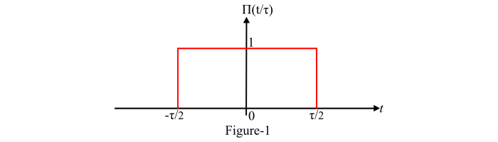
It is defined as,
$$\mathrm{rect\left(\frac{t}{\tau}\right)\:=\:\prod\left(\frac{t}{\tau}\right)\:=\:\begin{cases}1 & for\:|t|\:\leq \:\left(\frac{\tau}{2}\right)\\\\0\: &\: otherwise\end{cases}}$$
Given that
$$\mathrm{x(t)\:=\:\prod\left(\frac{t}{\tau}\right)}$$
Hence, from the definition of Fourier transform, we have,
$$\mathrm{F\left[\prod\left(\frac{t}{\tau}\right) \right]\:=\:X(\omega)\:=\:\int_{-\infty}^{\infty}x(t)e^{-j\omega t}\:dt\:=\:\int_{-\infty}^{\infty}\prod\left(\frac{t}{\tau}\right)e^{-j\omega t}\:dt}$$
$$\mathrm{\Rightarrow\:X(\omega)\:=\:\int_{-(\tau/2)}^{(\tau/2)}1\:\cdot\: e^{-j\omega t}\:dt\:=\:\left[\frac{e^{-j\omega t}}{-j\omega} \right]_{-\tau/2}^{\tau/2}}$$
$$\mathrm{\Rightarrow\:X(\omega)\:=\:\left[ \frac{e^{-j\omega (\tau/2)}\:-\:e^{j\omega (\tau/2)}}{-j\omega}\right]\:=\: \left[ \frac{e^{j\omega (\tau/2)}\:-\:e^{-j\omega (\tau/2)}}{j\omega }\right]}$$
$$\mathrm{\Rightarrow\:X(\omega)\:=\:\left[ \frac{2\tau[e^{j\omega (\tau/2)}\:-\:e^{-j\omega (\tau/2)}]}{j\omega\:\cdot\: (2\tau) }\right]\:=\:\frac{\tau}{\omega(\tau/2)}\left[\frac{e^{j\omega (\tau/2)}\:-\:e^{-j\omega (\tau/2)}}{2j} \right]}$$
$$\mathrm{\because \:\left[\frac{e^{j\omega (\tau/2)}\:-\:e^{-j\omega (\tau/2)}}{2j} \right]\:=\:sin\:\omega (\tau/2)}$$
$$\mathrm{\therefore\:X(\omega)\:=\:\frac{\tau}{\omega(\tau/2)}\:\cdot\: sin \omega (\tau/2)\:=\: \tau \left[\frac{ sin\omega (\tau/2)}{\omega (\tau/2)}\right]}$$
$$\mathrm{\because\:sinc \left(\frac{\omega \tau}{2}\right)\:=\:\frac{sin\omega (\tau/2)}{\omega (\tau/2)}}$$
$$\mathrm{\therefore\:X(\omega)\:=\: \tau\:\cdot\: sinc \left(\frac{\omega \tau}{2}\right)}$$
Therefore, the Fourier transform of the rectangular function is
$$\mathrm{F\left[\prod\left(\frac{t}{\tau}\right)\right]\:=\:\tau\:\cdot\: sinc \left(\frac{\omega \tau}{2}\right)}$$
Or, it can also be represented as,
$$\mathrm{\prod\left(\frac{t}{\tau}\right) \overset{FT}{\leftrightarrow}\tau\:\cdot\: sinc \left(\frac{\omega \tau}{2}\right)}$$
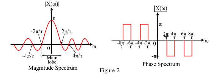
Magnitude and phase spectrum of Fourier transform of the rectangular function
The magnitude spectrum of the rectangular function is obtained as −
At $\omega\:=\:0$:
$$\mathrm{sinc\left(\frac{\omega \tau}{2}\right)\:=\:1;\:\:\Rightarrow\:|X(\omega)|\:=\:\tau}$$
At $\mathrm{\left(\frac{\omega \tau}{2}\right)\:=\:± n\pi}$ i.e., at
$$\mathrm{\omega=±\frac{2n\pi}{\tau},\:\:n=1,2,2,3,...}$$
$$\mathrm{sinc\left(\frac{\omega\: \tau}{2}\right)\:=\:0}$$
The phase spectrum is obtained as −
$$\mathrm{\angle\:X(\omega)\:=\:\begin{cases}0\: &\: if\:sinc\:\left(\frac{\omega \tau}{2}\right)\: \gt\: 0\:\\\\±\pi\: & \:if\:sinc\:\left(\frac{\omega \tau}{2}\right)\:\lt\: 0 \end{cases}}$$
The frequency spectrum of the rectangular function is shown in Figure-2.
Note
- The magnitude response between the first two zero crossings is known as the main lobe.
- The portions of the magnitude response for $\mathrm{\omega\:\lt\: -\left(\frac{-2\pi}{\tau}\right)}$ and $\mathrm{\omega \:\gt\: \left( \frac{2\pi}{\tau}\right)}$are known as the side lobes.
- From the magnitude spectrum, it is clear that the majority of the energy of the signal is contained in the main lobe.
- The main lobe becomes narrower with the increase in the width of the rectangular pulse.
- The phase spectrum of the rectangular function is an odd function of the frequency (ω).
- When the magnitude spectrum is positive, then the phase is zero and if the magnitude spectrum is negative, then the phase is $(±\pi)$.
