- Data Comm & Networks Home
- DCN - Overview
- DCN - What is Computer Network
- DCN - Uses of Computer Network
- DCN - Computer Network Types
- DCN - Network LAN Technologies
- DCN - Computer Network Models
- DCN - Computer Network Security
- DCN - Components
- DCN - Connectors
- DCN - Switches
- DCN - Repeaters
- DCN - Gateways
- DCN - Bridges
- DCN - Socket
- DCN - Network Interface Card
- DCN - NIC: Pros and Cons
- DCN - Network Hardware
- DCN - Network Port
- Computer Network Topologies
- DCN - Computer Network Topologies
- DCN - Point-to-point Topology
- DCN - Bus Topology
- DCN - Star Topology
- DCN - Ring Topology
- DCN - Mesh Topology
- DCN - Tree Topology
- DCN - Hybrid Topology
- Physical Layer
- DCN - Physical Layer Introduction
- DCN - Digital Transmission
- DCN - Analog Transmission
- DCN - Transmission media
- DCN - Wireless Transmission
- DCN - Transmission Impairments
- DCN - Multiplexing
- DCN - Network Switching
- DCN - Circuit Switching
- DCN - Packet Switching
- DCN - Message Switching
- Data Link Layer
- DCN - Data Link Layer Introduction
- DCN - Data Link Control & Protocols
- DCN - RMON
- DCN - Token Ring Network
- DCN - Hamming Code
- DCN - Byte Stuffing
- DCN - Channel Allocation
- DCN - MAC Address
- DCN - Address Resolution Protocol
- DCN - Cyclic Redundancy Checks
- DCN - Error Control
- DCN - Flow Control
- DCN - Framing
- DCN - Error Detection & Correction
- DCN - Error Correcting Codes
- DCN - Parity Bits
- Network Layer
- DCN - Network Layer Introduction
- DCN - Network Addressing
- DCN - Routing
- DCN - Routing Table
- DCN - Internetworking
- DCN - Network Layer Protocols
- DCN - Routing Information Protocol
- DCN - Border Gateway Protocol
- DCN - OSPF Protocol
- DCN - Network Address Translation
- DCN - Network Address Translation Types
- Transport Layer
- DCN - Transport Layer Introduction
- DCN - Transmission Control Protocol
- DCN - User Datagram Protocol
- DCN - Congestion Control
- DCN - Open Loop Congestion Control
- DCN - Closed Loop Congestion Control
- DCN - Congestion Control Algorithms
- DCN - Token Bucket Algorithm
- DCN - TCP Tahoe Algorithm
- DCN - TCP Reno Algorithm
- DCN - TCP New Reno Algorithm
- DCN - TCP BIC Algorithm
- DCN - TCP CUBIC Algorithm
- DCN - TCP Service Model
- DCN - TLS Handshake
- DCN - TCP Vs. UDP
- Application Layer
- DCN - Session Layer
- DCN - Presentation Layer
- DCN - Application Layer Introduction
- DCN - Client-Server Model
- DCN - Application Protocols
- DCN - Network Services
- DCN - Virtual Private Network
- DCN - Load Shedding
- DCN - Optimality Principle
- DCN - Service Primitives
- DCN - Services of Network Security
- DCN - Hypertext Transfer Protocol
- DCN - File Transfer Protocol
- DCN - Secure Socket Layer
- Network Protocols
- DCN - ALOHA Protocol
- DCN - Pure ALOHA Protocol
- DCN - Sliding Window Protocol
- DCN - Stop and Wait Protocol
- DCN - Link State Routing
- DCN - Link State Routing Protocol
- Network Algorithms
- DCN - Shortest Path Algorithm
- DCN - Routing Algorithm
- DCN - Adaptive Routing Algorithms
- DCN - Non-Adaptive Routing Algorithms
- DCN - Leaky Bucket Algorithm
- Wireless Networks
- DCN - Wireless Networks
- DCN - Wireless LANs
- DCN - Wireless LAN & IEEE 802.11
- DCN - IEEE 802.11 Wireless LAN Standards
- DCN - IEEE 802.11 Networks
- Multiplexing
- DCN - Multiplexing & Its Types
- DCN - Time Division Multiplexing
- DCN - Synchronous TDM
- DCN - Asynchronous TDM
- DCN - Synchronous Vs. Asynchronous TDM
- DCN - Frequency Division Multiplexing
- DCN - TDM Vs. FDM
- DCN - Code Division Multiplexing
- DCN - Wavelength Division Multiplexing
- Miscellaneous
- DCN - Shortest Path Routing
- DCN - B-ISDN Reference Model
- DCN - Design Issues For Layers
- DCN - Selective-repeat ARQ
- DCN - Flooding
- DCN - E-Mail Format
- DCN - Cryptography
- DCN - Unicast, Broadcast, & Multicast
- DCN - Network Virtualization
- DCN - Flow Vs. Congestion Control
- DCN - Asynchronous Transfer Mode
- DCN - ATM Networks
- DCN - Synchronous Vs. Asynchronous Transmission
- DCN - Network Attacks
- DCN - WiMax
- DCN - Buffering
- DCN - Authentication
- DCN Useful Resources
- DCN - Quick Guide
- DCN - Useful Resources
- DCN - Discussion
TCP CUBIC Congestion Control Algorithm
TCP CUBIC (CUBIC Congestion Control) is an advanced congestion control algorithm that improves the performance of TCP in high-speed and long-distance networks. It addresses the limitations of traditional TCP algorithms (like Reno and New Reno) and also is improvement of TCP BIC with better fairness and easy implementation.
TCP CUBIC congestion control algorithm uses a cubic function to find the growth of congestion window (cwnd). It adjusts the rate of sending packets using a cubic function of the time duration since the last congestion event. It makes the window growth independent of RTT (Round Trip Time).
TCP CUBIC improves the performance of fast networks where data takes more time to travel between sender and receiver, for example, long distance fiber networks. It provides better RTT-fairness and scalability in high speed networks than TCP Reno, New Reno, and BIC algorithms. It uses a function also called cubic window increase function that has three different phases: first is the concave region also known as fast recovery, the second is plateau region also called cautious probing, and the third is convex region also known as aggressive probing.
Earlier TCP algorithms like Reno and New Reno had limitations in high-speed networks. TCP BIC solved the limitations of Reno and New Reno but uses complex logic with multiple phases. TCP CUBIC uses a single cubic function and maintains the performance.
Here are the important characteristics of TCP CUBIC algorithm −
- It uses a cubic function for getting window growth and make it independent of RTT.
- Provides better RTT-fairness as compared to TCP BIC and other traditional TCP congestion control algorithms.
- Better stability and fast convergence with high bandwidth utilization.
Working of TCP CUBIC Algorithm
The following image depicts all the phases of TCP CUBIC algorithm −
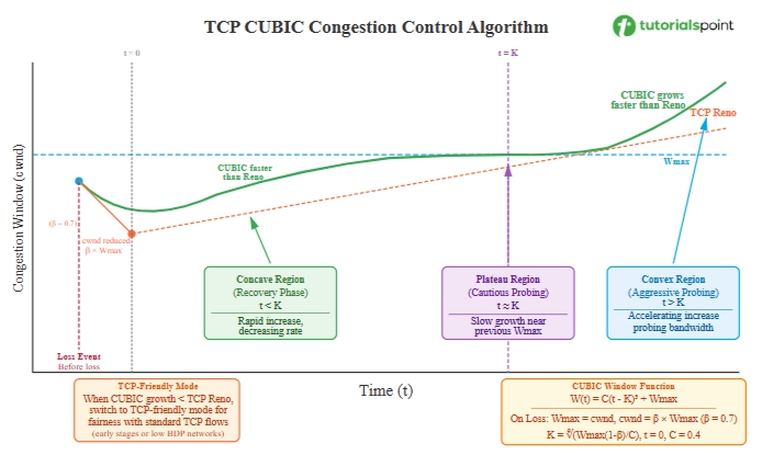
Let's now understand the working of TCP CUBIC algorithm in various phases −
Cubic Window Growth Function
The window growth function in CUBIC algorithm is given as: W(t) = C(t - K)3 + Wmax, where C represents scaling constant, t represents time passed since last window reduction, K represents time taken by function to increase W to Wmax, and Wmax represents window size before the last reduction.
Concave Region
Just after a loss event, when t < K, it represents the concave region of cubic function. In this region, the window increases quickly but at decreasing rate. This helps to recover quickly towards the previous Wmax value. It is also known as Fast Recovery region.
Plateau Region (Cautious Probing)
When t ≈ K, the window is near Wmax. The cubic function flattens out, so there is slow growth in this region. It helps in avoiding immediate congestion after reaching the previous maximum. It is also known as Cautious Probing region.
Convex Region (Aggressive Probing)
When t > K, after surpassing Wmax without loss, the function enters the convex region. This window increases at a very fast rate to probe for additional available bandwidth. It is also known as Aggressive Probing region.
TCP-Friendly Region
In TCP-Friendly region, the cubic function grows slower than TCP Reno. CUBIC algorithm switches to a TCP-friendly mode to ensure fairness with standard TCP flows.
Loss Handling
In case of packet loss, CUBIC algorithm does the following −
- It sets Wmax to the current cwnd.
- It reduces cwnd using multiplicative decrease to 70% of current cwnd (β = 0.7).
- It resets the timer t = 0.
- It calculates K = ((Wmax - cwnd)/C)1/3 for the new cubic iteration.
Example
Here is an example demonstrating TCP CUBIC behavior with packet loss. Initially, cwnd = 10, C = 0.4, β = 0.7
Initial State:
cwnd = 10, Wmax = undefined, C = 0.4, β = 0.7
RTT 1-4: Cubic growth (concave phase)
cwnd grows: 10 => 42 => 74 => 106
RTT 5: cwnd = 138, Packet loss occurs
=> Wmax = 138
=> cwnd = 138 * 0.7 = 97 (using β = 0.7)
=> K = ((138 - 97)/0.4)1/3 = (102.5)1/3 ≈ 4.68
=> t = 0
RTT 6: Concave phase begins (t = 1)
=> W(1) = 0.4(1 - 4.68)3 + 138 ≈ 118
=> cwnd = 118
RTT 7: Continuing concave growth (t = 2)
=> W(2) = 0.4(2 - 4.68)3 + 138 ≈ 130
=> cwnd = 130
RTT 8: Approaching plateau (t = 3)
=> W(3) = 0.4(3 - 4.68)3 + 138 ≈ 136
=> cwnd = 136
RTT 9: Near Wmax (t = 4)
=> W(4) = 0.4(4 - 4.68)3 + 138 ≈ 138
=> cwnd = 138
RTT 10: Plateau region (t = 5)
=> W(5) = 0.4(5 - 4.68)3 + 138 ≈ 138
=> cwnd = 138
RTT 11: Entering convex region (t = 6)
=> W(6) = 0.4(6 - 4.68)3 + 138 ≈ 139
=> cwnd = 139
RTT 12: Convex growth (t = 7), Packet loss occurs
=> Wmax = 139
=> cwnd = 139 * 0.7 = 97
=> K = ((139 - 97)/0.4)1/3 ≈ 4.71
=> t = 0
RTT 13: New epoch begins
=> W(1) = 0.4(1 - 4.71)3 + 139 ≈ 118
=> cwnd = 118
RTT 14: Concave growth
=> W(2) = 0.4(2 - 4.71)3 + 139 ≈ 131
=> cwnd = 131
Steps to Implement TCP CUBIC Algorithm
Here are the steps to implement TCP CUBIC algorithm −
- Initially, set cwnd = 1 MSS, initial ssthresh, cubic constant C = 0.4, β = 0.7, the number of iterations, and round at which the loss will occur i.e., 5 and 12.
- In Slow Start phase, increase cwnd by 1 MSS for each ACK received.
- When cwnd reaches ssthresh, switch to Congestion Avoidance phase using the CUBIC function.
- In case of packet loss, set Wmax = cwnd and reduce cwnd to cwnd * β (where β = 0.7).
- Calculate the value of K using ((Wmax - cwnd)/C)1/3 and reset the time to t = 0.
- Calculate target window using W(t) = C(t - K)3 + Wmax for each RTT in Congestion Avoidance phase.
- In the concave phase when (t < K), cwnd increases quickly toward Wmax.
- In the plateau region phase when (t ≈ K), cwnd growth slows down for cautious probing.
- In the convex region phase when (t > K), cwnd increases quickly to probe for more bandwidth.
- Implement TCP-friendly mode. If CUBIC growth becomes slower than TCP Reno, then use Reno's growth rate in place of CUBIC growth.
- In case of timeout, reset cwnd to 1 MSS, set Wmax = 0, and restart from Slow Start.
Code Implementation
Here is the code implementation of the above steps for TCP CUBIC algorithm in C++, Java, and Python −
#include <iostream>
#include <cmath>
#include <algorithm>
using namespace std;
class TCPCUBIC {
private:
    double cwnd;
    double wmax;
    double C;
    double beta;
    int t;
    double K;
    bool tcp_friendly;
public:
    TCPCUBIC(double init_cwnd = 10.0, double cubic_c = 0.4,
             double b = 0.7, bool tf = true) {
        cwnd = init_cwnd;
        wmax = 0.0;
        C = cubic_c;
        beta = b;
        t = 0;
        K = 0.0;
        tcp_friendly = tf;
    }
    void onAck() {
        t++;

        if (wmax == 0.0) {
            // No previous loss, use simple growth
            cwnd += 1.0;
        } else {
            // CUBIC function: W(t) = C(t-K)^3 + Wmax
            double time_diff = t - K;
            double target = C * pow(time_diff, 3) + wmax;

            // TCP-friendly mode check
            double tcp_cwnd = cwnd + (3 * beta) / (2 - beta) * (t / cwnd);

            if (tcp_friendly && target < tcp_cwnd) {
                cwnd = tcp_cwnd;
            } else {
                cwnd = target;
            }

            // Ensure cwnd doesn't decrease
            if (cwnd < wmax * beta) {
                cwnd = wmax * beta;
            }
        }
    }
    void onLoss() {
        wmax = cwnd;
        cwnd = cwnd * beta;
        t = 0;

        // Calculate K: time to reach Wmax again
        K = cbrt((wmax - cwnd) / C);
    }
    double getCwnd() { return cwnd; }
    double getWmax() { return wmax; }

    void printState(int rtt) {
        cout << rtt << "\t" << (int)cwnd << "\t\t" << (int)wmax
             << "\t\t" << t << endl;
    }
};
int main() {
    TCPCUBIC cubic(10.0);
    int maxRTT = 15;
    int lossRound1 = 5;
    int lossRound2 = 12;

    cout << "RTT\tcwnd\t\tWmax\t\tTime(t)" << endl;

    for (int r = 1; r <= maxRTT; r++) {
        cubic.printState(r);

        if (r == lossRound1) {
            cout << "=> Packet loss detected at RTT " << r << endl;
            cubic.onLoss();
            cout << "=> cwnd reduced, Wmax updated, epoch reset" << endl;
        } else if (r == lossRound2) {
            cout << "=> Packet loss detected at RTT " << r << endl;
            cubic.onLoss();
            cout << "=> cwnd reduced, new epoch begins" << endl;
        } else {
            cubic.onAck();
        }
    }

    return 0;
}
The output of the above code is as follows −
RTT	cwnd		Wmax		Time(t)
1	10		0		0
2	11		0		1
3	12		0		2
4	13		0		3
5	14		0		4
=> Packet loss detected at RTT 5
=> cwnd reduced, Wmax updated, epoch reset
6	9		14		0
7	11		14		1
8	12		14		2
9	13		14		3
10	14		14		4
11	14		14		5
12	14		14		6
=> Packet loss detected at RTT 12
=> cwnd reduced, new epoch begins
13	9		14		0
14	11		14		1
15	12		14		2
class TCPCUBIC {
    private double cwnd;
    private double wmax;
    private double C;
    private double beta;
    private int t;
    private double K;
    private boolean tcpFriendly;
    public TCPCUBIC(double initCwnd, double cubicC, double b, boolean tf) {
        this.cwnd = initCwnd;
        this.wmax = 0.0;
        this.C = cubicC;
        this.beta = b;
        this.t = 0;
        this.K = 0.0;
        this.tcpFriendly = tf;
    }
    public void onAck() {
        t++;

        if (wmax == 0.0) {
            cwnd += 1.0;
        } else {
            // CUBIC function
            double timeDiff = t - K;
            double target = C * Math.pow(timeDiff, 3) + wmax;

            // TCP-friendly check
            double tcpCwnd = cwnd + (3 * beta) / (2 - beta) * (t / cwnd);

            if (tcpFriendly && target < tcpCwnd) {
                cwnd = tcpCwnd;
            } else {
                cwnd = target;
            }

            if (cwnd < wmax * beta) {
                cwnd = wmax * beta;
            }
        }
    }
    public void onLoss() {
        wmax = cwnd;
        cwnd = cwnd * beta;
        t = 0;
        K = Math.cbrt((wmax - cwnd) / C);
    }
    public double getCwnd() { return cwnd; }
    public double getWmax() { return wmax; }

    public void printState(int rtt) {
        System.out.println(rtt + "\t" + (int)cwnd + "\t\t" + (int)wmax
                         + "\t\t" + t);
    }
}
public class Main {
    public static void main(String[] args) {
        TCPCUBIC cubic = new TCPCUBIC(10.0, 0.4, 0.7, true);
        int maxRTT = 15;
        int lossRound1 = 5;
        int lossRound2 = 12;

        System.out.println("RTT\tcwnd\t\tWmax\t\tTime(t)");

        for (int r = 1; r <= maxRTT; r++) {
            cubic.printState(r);

            if (r == lossRound1) {
                System.out.println("=> Packet loss detected at RTT " + r);
                cubic.onLoss();
                System.out.println("=> cwnd reduced, Wmax updated, epoch reset");
            } else if (r == lossRound2) {
                System.out.println("=> Packet loss detected at RTT " + r);
                cubic.onLoss();
                System.out.println("=> cwnd reduced, new epoch begins");
            } else {
                cubic.onAck();
            }
        }
    }
}
The output of the above code is as follows −
RTT	cwnd		Wmax		Time(t)
1	10		0		0
2	11		0		1
3	12		0		2
4	13		0		3
5	14		0		4
=> Packet loss detected at RTT 5
=> cwnd reduced, Wmax updated, epoch reset
6	9		14		0
7	11		14		1
8	12		14		2
9	13		14		3
10	14		14		4
11	14		14		5
12	14		14		6
=> Packet loss detected at RTT 12
=> cwnd reduced, new epoch begins
13	9		14		0
14	11		14		1
15	12		14		2
class TCPCUBIC:
    def __init__(self, init_cwnd=10.0, cubic_c=0.4, beta=0.7, tcp_friendly=True):
        self.cwnd = init_cwnd
        self.wmax = 0.0
        self.C = cubic_c
        self.beta = beta
        self.t = 0
        self.K = 0.0
        self.tcp_friendly = tcp_friendly
    def on_ack(self):
        self.t += 1

        if self.wmax == 0.0:
            self.cwnd += 1.0
        else:
            # CUBIC function: W(t) = C(t-K)^3 + Wmax
            time_diff = self.t - self.K
            target = self.C * (time_diff ** 3) + self.wmax

            # TCP-friendly mode
            tcp_cwnd = self.cwnd + (3 * self.beta) / (2 - self.beta) * (self.t / self.cwnd)

            if self.tcp_friendly and target < tcp_cwnd:
                self.cwnd = tcp_cwnd
            else:
                self.cwnd = target

            if self.cwnd < self.wmax * self.beta:
                self.cwnd = self.wmax * self.beta
    def on_loss(self):
        self.wmax = self.cwnd
        self.cwnd = self.cwnd * self.beta
        self.t = 0
        self.K = ((self.wmax - self.cwnd) / self.C) ** (1/3)
    def print_state(self, rtt):
        print(f"{rtt}\t{int(self.cwnd)}\t\t{int(self.wmax)}\t\t{self.t}")
def simulate():
    cubic = TCPCUBIC(init_cwnd=10.0)
    max_rtt = 15
    loss_round1 = 5
    loss_round2 = 12

    print("RTT\tcwnd\t\tWmax\t\tTime(t)")

    for r in range(1, max_rtt + 1):
        cubic.print_state(r)

        if r == loss_round1:
            print(f"=> Packet loss detected at RTT {r}")
            cubic.on_loss()
            print("=> cwnd reduced, Wmax updated, epoch reset")
        elif r == loss_round2:
            print(f"=> Packet loss detected at RTT {r}")
            cubic.on_loss()
            print("=> cwnd reduced, new epoch begins")
        else:
            cubic.on_ack()
if __name__ == "__main__":
    simulate()
The output of the above code is as follows −
RTT	cwnd		Wmax		Time(t)
1	10		0		0
2	11		0		1
3	12		0		2
4	13		0		3
5	14		0		4
=> Packet loss detected at RTT 5
=> cwnd reduced, Wmax updated, epoch reset
6	9		14		0
7	11		14		1
8	12		14		2
9	13		14		3
10	14		14		4
11	14		14		5
12	14		14		6
=> Packet loss detected at RTT 12
=> cwnd reduced, new epoch begins
13	9		14		0
14	11		14		1
15	12		14		2
Pros and Cons of TCP CUBIC Algorithm
The advantages of TCP CUBIC algorithm are as follows −
- Better scalability in high bandwidth-delay product networks.
- Window growth does not depend on RTT which makes bandwidth sharing fair.
- Simpler implementation than TCP BIC since CUBIC has single cubic function.
Here are the limitations of TCP CUBIC algorithm −
- In some network conditions, it leads to packet loss.
- It requires accurate RTT measurements for better performance.
- Complex computation.
Difference between TCP BIC and TCP CUBIC Algorithm
The follwing table highlights the major differences between TCP BIC and TCP CUBIC algorithms −
| TCP BIC Algorithm | TCP CUBIC Algorithm |
|---|---|
| It uses binary search with multiple phases. | It uses a single cubic function for all phases. |
| Window growth depends on RTT. | Window growth is RTT independent. |
| Complex implementation with phase transitions. | Simpler implementation with single cubic function. |
| It reduces cwnd to 80% on packet loss. | It reduces cwnd to 70% on packet loss. |
| There is no TCP friendly mode. | It has TCP friendly mode. |
Conclusion
TCP CUBIC congestion control algorithm uses a cubic function for adjusting the congestion window (cwnd) over time; it provides better performance in high-speed networks. TCP CUBIC is an improvement of TCP BIC with simpler implementation, better RTT-fairness, uses TCP-friendly mode.
