- Data Comm & Networks Home
- DCN - Overview
- DCN - What is Computer Network
- DCN - Uses of Computer Network
- DCN - Computer Network Types
- DCN - Network LAN Technologies
- DCN - Computer Network Models
- DCN - Computer Network Security
- DCN - Components
- DCN - Connectors
- DCN - Switches
- DCN - Repeaters
- DCN - Gateways
- DCN - Bridges
- DCN - Socket
- DCN - Network Interface Card
- DCN - NIC: Pros and Cons
- DCN - Network Hardware
- DCN - Network Port
- Computer Network Topologies
- DCN - Computer Network Topologies
- DCN - Point-to-point Topology
- DCN - Bus Topology
- DCN - Star Topology
- DCN - Ring Topology
- DCN - Mesh Topology
- DCN - Tree Topology
- DCN - Hybrid Topology
- Physical Layer
- DCN - Physical Layer Introduction
- DCN - Digital Transmission
- DCN - Analog Transmission
- DCN - Transmission media
- DCN - Wireless Transmission
- DCN - Transmission Impairments
- DCN - Multiplexing
- DCN - Network Switching
- DCN - Circuit Switching
- DCN - Packet Switching
- DCN - Message Switching
- Data Link Layer
- DCN - Data Link Layer Introduction
- DCN - Data Link Control & Protocols
- DCN - RMON
- DCN - Token Ring Network
- DCN - Hamming Code
- DCN - Byte Stuffing
- DCN - Channel Allocation
- DCN - MAC Address
- DCN - Address Resolution Protocol
- DCN - Cyclic Redundancy Checks
- DCN - Error Control
- DCN - Flow Control
- DCN - Framing
- DCN - Error Detection & Correction
- DCN - Error Correcting Codes
- DCN - Parity Bits
- Network Layer
- DCN - Network Layer Introduction
- DCN - Network Addressing
- DCN - Routing
- DCN - Routing Table
- DCN - Internetworking
- DCN - Network Layer Protocols
- DCN - Routing Information Protocol
- DCN - Border Gateway Protocol
- DCN - OSPF Protocol
- DCN - Network Address Translation
- DCN - Network Address Translation Types
- Transport Layer
- DCN - Transport Layer Introduction
- DCN - Transmission Control Protocol
- DCN - User Datagram Protocol
- DCN - Congestion Control
- DCN - Open Loop Congestion Control
- DCN - Closed Loop Congestion Control
- DCN - Congestion Control Algorithms
- DCN - Token Bucket Algorithm
- DCN - TCP Tahoe Algorithm
- DCN - TCP Reno Algorithm
- DCN - TCP New Reno Algorithm
- DCN - TCP BIC Algorithm
- DCN - TCP CUBIC Algorithm
- DCN - TCP Service Model
- DCN - TLS Handshake
- DCN - TCP Vs. UDP
- Application Layer
- DCN - Session Layer
- DCN - Presentation Layer
- DCN - Application Layer Introduction
- DCN - Client-Server Model
- DCN - Application Protocols
- DCN - Network Services
- DCN - Virtual Private Network
- DCN - Load Shedding
- DCN - Optimality Principle
- DCN - Service Primitives
- DCN - Services of Network Security
- DCN - Hypertext Transfer Protocol
- DCN - File Transfer Protocol
- DCN - Secure Socket Layer
- Network Protocols
- DCN - ALOHA Protocol
- DCN - Pure ALOHA Protocol
- DCN - Sliding Window Protocol
- DCN - Stop and Wait Protocol
- DCN - Link State Routing
- DCN - Link State Routing Protocol
- Network Algorithms
- DCN - Shortest Path Algorithm
- DCN - Routing Algorithm
- DCN - Adaptive Routing Algorithms
- DCN - Non-Adaptive Routing Algorithms
- DCN - Leaky Bucket Algorithm
- Wireless Networks
- DCN - Wireless Networks
- DCN - Wireless LANs
- DCN - Wireless LAN & IEEE 802.11
- DCN - IEEE 802.11 Wireless LAN Standards
- DCN - IEEE 802.11 Networks
- Multiplexing
- DCN - Multiplexing & Its Types
- DCN - Time Division Multiplexing
- DCN - Synchronous TDM
- DCN - Asynchronous TDM
- DCN - Synchronous Vs. Asynchronous TDM
- DCN - Frequency Division Multiplexing
- DCN - TDM Vs. FDM
- DCN - Code Division Multiplexing
- DCN - Wavelength Division Multiplexing
- Miscellaneous
- DCN - Shortest Path Routing
- DCN - B-ISDN Reference Model
- DCN - Design Issues For Layers
- DCN - Selective-repeat ARQ
- DCN - Flooding
- DCN - E-Mail Format
- DCN - Cryptography
- DCN - Unicast, Broadcast, & Multicast
- DCN - Network Virtualization
- DCN - Flow Vs. Congestion Control
- DCN - Asynchronous Transfer Mode
- DCN - ATM Networks
- DCN - Synchronous Vs. Asynchronous Transmission
- DCN - Network Attacks
- DCN - WiMax
- DCN - Buffering
- DCN - Authentication
- DCN Useful Resources
- DCN - Quick Guide
- DCN - Useful Resources
- DCN - Discussion
Adaptive Routing Algorithm
Routing helps data packets travel from source to destination. A routing algorithm is a procedure that mathematically computes the best path or route to transfer data packets from source to the destination. They direct internet traffic efficiently. After a data packet leaves its source, it can choose among various paths to reach its destination.
Routing algorithms are broadly categorized into two types: adaptive and non-adaptive routing algorithms. Read this chapter to understand Adaptive Routing Algorithms in detail.
What is Adaptive Routing Algorithm?
Adaptive routing algorithms, also known as dynamic routing algorithms, makes routing decisions dynamically while transferring data packets from the source to the destination. These algorithms constructs routing tables depending on the network conditions like network traffic and topology. They try to find the best path or least cost path, depending upon the hop count, transit time and distance.
Routes are dynamically updated in the following conditions: topology changes, link failures, or traffic variations. The path changes dynamically based on current network traffic, congestion, and topology conditions. Routers share information and update their routing tables dynamically to adapt to changing network conditions.
The routing table is automatically updated based on network conditions and routing protocols. It uses routing algorithms like distance vector or link state that provide dynamic adaptability. Dynamic routing is mainly used in large and complex networks. It can dynamically find alternative paths when link failures occur.
How Do Adaptive Routing Algorithms Work?
In the following list of points, we explain how adaptive routing algorithms works −
- The routers continuously monitor the link status, bandwidth availability, delay, and congestion levels.
- Each router uses routing protocols to collect information about its neighbors and network topology.
- Routers share information with their neighboring routers or a central controller for updating their routing table.
- Next, the routers calculate the best paths to reach their destinations using various algorithms like Dijkstra's or Bellman-Ford.
- Thereafter, the routing tables are updated dynamically.
- Based on the optimal path determined by the routing table, the data packets are forwarded.
Characteristics of Adaptive Routing Algorithm
The key characteristics of dynamic routing are given below −
- In dynamic routing, routes are changed dynamically based on network conditions.
- It is complex to implement and maintain.
- Routes are dynamically computed by routing protocols like BGP, RIP and EIGRP.
- Higher computational overhead since resources are continuously monitored and updated.
- The routing table is dynamic and updates automatically.
- There is continuous real-time monitoring of network conditions.
Types of Adaptive Routing Algorithms
There are three main types of adaptive or dynamic routing algorithms that are mentioned below −
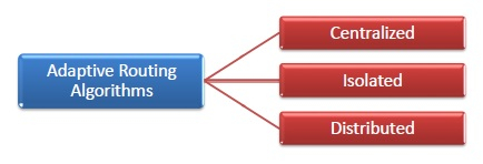
Centralized Routing
In centralized routing, one centralized node has the total network information and takes the routing decisions. It finds the least-cost path between source and destination nodes by using global knowledge about the network.
The advantage of centralized routing is that only the central node is required to store network information and so the resource requirement of the other nodes may be less. However, routing performance is too much dependent upon the central node. Example of centralized routing is: Software-Defined Networking (SDN) controllers.
The advantages of centralized routing are as follows −
- It has complete information of total network that helps in choosing optimal paths.
- Easier network management.
- Easy troubleshooting.
- Since a central node takes routing decision, therefore no complex algorithms is needed for routers.
The disadvantages of centralized routing are given below −
- If the central node fails, complete network fails.
- It is not scalable as it can not be used in very large networks.
- Communication overhead with central controller.
- There is delay in response to network changes.
Isolated Routing
In isolated routing algorithm, the nodes make the routing decisions based upon local information available to them instead of gathering information from other nodes. They do not have information regarding the link status. While this helps in fast decision making, the nodes may transmit data packets along congested network resulting in delay. The examples of isolated routing are hot potato routing and backward learning.
Hot Potato Routing Algorithm
Hot potato routing is a simple routing technique in which each node tries to get rid of packets as soon as possible. When a packet arrives at a node, it is immediately forwarded to the first available outgoing link.
Network congestion or optimal path is not considered in this case. The node selects the shortest length to forward the packet. It is treated like a hot potato which is passed on quickly.
Backward Learning Algorithm
In backward learning, nodes learn about network topology. Nodes analyzes the incoming packets for learning network topology. When a packet arrives from a source, the receiving node stores the path information and then uses it to send back the packets to that source later on. It builds routing tables based on the reverse path of received packets.
The advantages of isolated routing are given below −
- Simple to implement and it requires less processing.
- Fast routing decisions because of local information only.
- There is no communication overhead between routers.
- Low memory requirements at each node.
- It can quickly respond to local conditions.
The disadvantages of isolated routing are given below −
- May not always give optimal routing paths.
- It can not adapt to global network conditions.
- Packets may be sent through congested links.
- It is not good for complex network topologies.
Distributed Routing
In distributed routing, each node receives information from its neighboring nodes and takes the decision based upon the received information. The least-cost path between source and destination is computed iteratively in a distributed manner.
An advantage is that each node can dynamically change routing decisions based upon the changes in the network. However, on the flip side, delays may be introduced due to time required to gather information. Example of distributed algorithm is distance vector and link state routing algorithm.
Distance Vector Routing
In distance vector routing, each router maintains their own routing table that stores the cost to reach every destination and the next hop to reach that destination. Routers share their routing tables with their immediate neighbors. Each router updates its routing table based on information from neighbors.
The distance metric are: hop count, delay, bandwidth, etc. An example of distance vector routing is Bellman-Ford algorithm. RIP (Routing Information Protocol), IGRP (Interior Gateway Routing Protocol), and EIGRP (Enhanced IGRP) are examples of distance vector routing protocols.
Here's an example code snippet for the Bellman-Ford Shortest Path algorithm in C, C++, Java, and Python −
#include <stdio.h>
#include <stdlib.h>
#include <limits.h>

#define MAX_VERTICES 6

int graph[MAX_VERTICES][MAX_VERTICES] = {
   {0, 10, 0, 15, 0, 0},
   {0, 0, 0, 5, 10, 0},
   {0, 0, 0, 0, 0, 10},
   {0, 0, 0, 0, 0, 5},
   {0, 0, 0, 0, 0, 10},
   {0, 0, 0, 0, 0, 0}
};

void bellman_ford(int source) {
   int distance[MAX_VERTICES];

   for (int i = 0; i < MAX_VERTICES; i++) {
      distance[i] = INT_MAX;
   }
   distance[source] = 0;

   for (int i = 0; i < MAX_VERTICES - 1; i++) {
      for (int u = 0; u < MAX_VERTICES; u++) {
         for (int v = 0; v < MAX_VERTICES; v++) {
            if (graph[u][v] != 0 && distance[u] != INT_MAX && distance[u] + graph[u][v] < distance[v]) {
               distance[v] = distance[u] + graph[u][v];
            }
         }
      }
   }

   for (int u = 0; u < MAX_VERTICES; u++) {
      for (int v = 0; v < MAX_VERTICES; v++) {
         if (graph[u][v] != 0 && distance[u] != INT_MAX && distance[u] + graph[u][v] < distance[v]) {
            printf("Graph contains negative weight cycle\n");
            return;
         }
      }
   }

   printf("Vertex   Distance from Source\n");
   for (int i = 0; i < MAX_VERTICES; i++) {
      if (distance[i] == INT_MAX)
         printf("%d \t\t INF\n", i);
      else
         printf("%d \t\t %d\n", i, distance[i]);
   }
}

int main() {
   bellman_ford(0);
   return 0;
}
Output
Following is the output of the above code −
Vertex   Distance from Source
0 		 0
1 		 10
2 		 INF
3 		 15
4 		 20
5 		 20
#include <iostream>
#include <climits>
using namespace std;

#define MAX_VERTICES 6

int graph[MAX_VERTICES][MAX_VERTICES] = {
   {0, 10, 0, 15, 0, 0},
   {0, 0, 0, 5, 10, 0},
   {0, 0, 0, 0, 0, 10},
   {0, 0, 0, 0, 0, 5},
   {0, 0, 0, 0, 0, 10},
   {0, 0, 0, 0, 0, 0}
};

void bellman_ford(int source) {
   int distance[MAX_VERTICES];

   for (int i = 0; i < MAX_VERTICES; i++) {
      distance[i] = INT_MAX;
   }
   distance[source] = 0;

   for (int i = 0; i < MAX_VERTICES - 1; i++) {
      for (int u = 0; u < MAX_VERTICES; u++) {
         for (int v = 0; v < MAX_VERTICES; v++) {
            if (graph[u][v] != 0 && distance[u] != INT_MAX && distance[u] + graph[u][v] < distance[v]) {
               distance[v] = distance[u] + graph[u][v];
            }
         }
      }
   }

   for (int u = 0; u < MAX_VERTICES; u++) {
      for (int v = 0; v < MAX_VERTICES; v++) {
         if (graph[u][v] != 0 && distance[u] != INT_MAX && distance[u] + graph[u][v] < distance[v]) {
            cout << "Graph contains negative weight cycle" << endl;
            return;
         }
      }
   }

   cout << "Vertex   Distance from Source" << endl;
   for (int i = 0; i < MAX_VERTICES; i++) {
      if (distance[i] == INT_MAX)
         cout << i << " \t\t INF" << endl;
      else
         cout << i << " \t\t " << distance[i] << endl;
   }
}

int main() {
   bellman_ford(0);
   return 0;
}
Output
Following is the output of the above code −
Vertex   Distance from Source
0 		 0
1 		 10
2 		 INF
3 		 15
4 		 20
5 		 20
// Java program to find the shortest path from a source node to all other nodes using Bellman-Ford algorithm
import java.util.*;

public class Main {
   static final int MAX_VERTICES = 6;
   static int[][] graph = {
      {0, 10, 0, 15, 0, 0},
      {0, 0, 0, 5, 10, 0},
      {0, 0, 0, 0, 0, 10},
      {0, 0, 0, 0, 0, 5},
      {0, 0, 0, 0, 0, 10},
      {0, 0, 0, 0, 0, 0}
   };

   static void bellmanFord(int source) {
      int[] distance = new int[MAX_VERTICES];

      for (int i = 0; i < MAX_VERTICES; i++) {
         distance[i] = Integer.MAX_VALUE;
      }
      distance[source] = 0;

      for (int i = 0; i < MAX_VERTICES - 1; i++) {
         for (int u = 0; u < MAX_VERTICES; u++) {
            for (int v = 0; v < MAX_VERTICES; v++) {
               if (graph[u][v] != 0 && distance[u] != Integer.MAX_VALUE && distance[u] + graph[u][v] < distance[v]) {
                  distance[v] = distance[u] + graph[u][v];
               }
            }
         }
      }

      for (int u = 0; u < MAX_VERTICES; u++) {
         for (int v = 0; v < MAX_VERTICES; v++) {
            if (graph[u][v] != 0 && distance[u] != Integer.MAX_VALUE && distance[u] + graph[u][v] < distance[v]) {
               System.out.println("Graph contains negative weight cycle");
               return;
            }
         }
      }

      System.out.println("Vertex   Distance from Source");
      for (int i = 0; i < MAX_VERTICES; i++) {
         if (distance[i] == Integer.MAX_VALUE)
            System.out.println(i + " \t\t INF");
         else
            System.out.println(i + " \t\t " + distance[i]);
      }
   }

    public static void main(String[] args) {
        bellmanFord(0);
    }

}
Output
Following is the output of the above code −
Vertex   Distance from Source
0 		 0
1 		 10
2 		 INF
3 		 15
4 		 20
5 		 20
MAX_VERTICES = 6

graph = [
    [0, 10, 0, 15, 0, 0],
    [0, 0, 0, 5, 10, 0],
    [0, 0, 0, 0, 0, 10],
    [0, 0, 0, 0, 0, 5],
    [0, 0, 0, 0, 0, 10],
    [0, 0, 0, 0, 0, 0]
]

def bellman_ford(source):
    distance = [float('inf')] * MAX_VERTICES
    distance[source] = 0

    # Relax all edges (V-1) times
    for i in range(MAX_VERTICES - 1):
        for u in range(MAX_VERTICES):
            for v in range(MAX_VERTICES):
                if graph[u][v] != 0 and distance[u] != float('inf'):
                    if distance[u] + graph[u][v] < distance[v]:
                        distance[v] = distance[u] + graph[u][v]

    # Print shortest distances
    print("Vertex\tDistance from Source")
    for i in range(MAX_VERTICES):
        print(f"{i}\t{distance[i]}")

# Example execution
bellman_ford(0)
Output
Following is the output of the above code −
Vertex   Distance from Source
0 		 0
1 		 10
2 		 INF
3 		 15
4 		 20
5 		 20
Link State Routing
In link state routing, each router maintains map of the network topology. Routers exchange information with all other routers instead of just neighbors. It provides more accurate routing compared to distance vector routing.
An example of link state routing algorithm is Dijkstra's algorithm OSPF (Open Shortest Path First) and IS-IS (Intermediate System to Intermediate System) are examples of link state routing protocols.
The dijkstra's algorithm finds the shortest path between two routers in a network. These two routers could either be adjacent or the farthest points in the network. Here is an example code of Dijkstra's Shortest Path algorithm in C, C++, Java, and Python −
#include<stdio.h>
#include<limits.h>
#include<stdbool.h>
int min_dist(int[], bool[]);
void greedy_dijsktra(int[][6],int);
int min_dist(int dist[], bool visited[]){ // finding minimum dist
   int minimum=INT_MAX,ind;
   for(int k=0; k<6; k++) {
      if(visited[k]==false && dist[k]<=minimum) {
         minimum=dist[k];
         ind=k;
      }
   }
   return ind;
}
void greedy_dijsktra(int graph[6][6],int src){
   int dist[6];
   bool visited[6];
   for(int k = 0; k<6; k++) {
      dist[k] = INT_MAX;
      visited[k] = false;
   }
   dist[src] = 0; // Source vertex dist is set 0
   for(int k = 0; k<6; k++) {
      int m=min_dist(dist,visited);
      visited[m]=true;
      for(int k = 0; k<6; k++) {

         // updating the dist of neighbouring vertex
         if(!visited[k] && graph[m][k] && dist[m]!=INT_MAX && dist[m]+graph[m][k]<dist[k])
            dist[k]=dist[m]+graph[m][k];
      }
   }
   printf("Vertex\t\tdist from source vertex\n");
   for(int k = 0; k<6; k++) {
      char str=65+k;
      printf("%c\t\t\t%d\n", str, dist[k]);
   }
}
int main(){
   int graph[6][6]= {
      {0, 1, 2, 0, 0, 0},
      {1, 0, 0, 5, 1, 0},
      {2, 0, 0, 2, 3, 0},
      {0, 5, 2, 0, 2, 2},
      {0, 1, 3, 2, 0, 1},
      {0, 0, 0, 2, 1, 0}
   };
   greedy_dijsktra(graph,0);
   return 0;
}
Output
Vertex		dist from source vertex
A			   0
B			   1
C			   2
D			   4
E			   2
F			   3
#include<iostream>
#include<climits>
using namespace std;
int min_dist(int dist[], bool visited[]){ // finding minimum dist
   int minimum=INT_MAX,ind;
   for(int k=0; k<6; k++) {
      if(visited[k]==false && dist[k]<=minimum) {
         minimum=dist[k];
         ind=k;
      }
   }
   return ind;
}
void greedy_dijsktra(int graph[6][6],int src){
   int dist[6];
   bool visited[6];
   for(int k = 0; k<6; k++) {
      dist[k] = INT_MAX;
      visited[k] = false;
   }
   dist[src] = 0; // Source vertex dist is set 0
   for(int k = 0; k<6; k++) {
      int m=min_dist(dist,visited);
      visited[m]=true;
      for(int k = 0; k<6; k++) {

         // updating the dist of neighbouring vertex
         if(!visited[k] && graph[m][k] && dist[m]!=INT_MAX && dist[m]+graph[m][k]<dist[k])
            dist[k]=dist[m]+graph[m][k];
      }
   }
   cout<<"Vertex\t\tdist from source vertex"<<endl;
   for(int k = 0; k<6; k++) {
      char str=65+k;
      cout<<str<<"\t\t\t"<<dist[k]<<endl;
   }
}
int main(){
   int graph[6][6]= {
      {0, 1, 2, 0, 0, 0},
      {1, 0, 0, 5, 1, 0},
      {2, 0, 0, 2, 3, 0},
      {0, 5, 2, 0, 2, 2},
      {0, 1, 3, 2, 0, 1},
      {0, 0, 0, 2, 1, 0}
   };
   greedy_dijsktra(graph,0);
   return 0;
}
Output
Vertex		dist from source vertex
A			   0
B			   1
C			   2
D			   4
E			   2
F			   3
public class Main {
   static int min_dist(int dist[], boolean visited[]) { // finding minimum dist
      int minimum = Integer.MAX_VALUE;
      int ind = -1;
      for (int k = 0; k < 6; k++) {
         if (!visited[k] && dist[k] <= minimum) {
            minimum = dist[k];
            ind = k;
         }
      }
      return ind;
   }
   static void greedy_dijkstra(int graph[][], int src) {
      int dist[] = new int[6];
      boolean visited[] = new boolean[6];
      for (int k = 0; k < 6; k++) {
         dist[k] = Integer.MAX_VALUE;
         visited[k] = false;
      }
      dist[src] = 0; // Source vertex dist is set 0
      for (int k = 0; k < 6; k++) {
         int m = min_dist(dist, visited);
         visited[m] = true;
         for (int j = 0; j < 6; j++) {
            // updating the dist of neighboring vertex
            if (!visited[j] && graph[m][j] != 0 && dist[m] != Integer.MAX_VALUE
                  && dist[m] + graph[m][j] < dist[j])
               dist[j] = dist[m] + graph[m][j];
         }
      }
      System.out.println("Vertex\t\tdist from source vertex");
      for (int k = 0; k < 6; k++) {
         char str = (char) (65 + k);
         System.out.println(str + "\t\t\t" + dist[k]);
      }
   }
   public static void main(String args[]) {
      int graph[][] = { { 0, 1, 2, 0, 0, 0 }, { 1, 0, 0, 5, 1, 0 }, { 2, 0, 0, 2, 3, 0 },
            { 0, 5, 2, 0, 2, 2 }, { 0, 1, 3, 2, 0, 1 }, { 0, 0, 0, 2, 1, 0 } };
      greedy_dijkstra(graph, 0);
   }
}
Output
Vertex		dist from source vertex
A			0
B			1
C			2
D			4
E			2
F			3
import sys
def min_dist(dist, visited):  # finding minimum dist
    minimum = sys.maxsize
    ind = -1
    for k in range(6):
        if not visited[k] and dist[k] <= minimum:
            minimum = dist[k]
            ind = k
    return ind
def greedy_dijkstra(graph, src):
    dist = [sys.maxsize] * 6
    visited = [False] * 6
    dist[src] = 0  # Source vertex dist is set 0
    for _ in range(6):
        m = min_dist(dist, visited)
        visited[m] = True
        for k in range(6):
            #  updating the dist of neighbouring vertex
            if not visited[k] and graph[m][k] and dist[m] != sys.maxsize and dist[m] + graph[m][k] < dist[k]:
                dist[k] = dist[m] + graph[m][k]
    print("Vertex\t\tdist from source vertex")
    for k in range(6):
        str_val = chr(65 + k)  # Convert index to corresponding character
        print(str_val, "\t\t\t", dist[k])
# Main code
graph = [
    [0, 1, 2, 0, 0, 0],
    [1, 0, 0, 5, 1, 0],
    [2, 0, 0, 2, 3, 0],
    [0, 5, 2, 0, 2, 2],
    [0, 1, 3, 2, 0, 1],
    [0, 0, 0, 2, 1, 0]
]
greedy_dijkstra(graph, 0)
Output
Vertex		dist from source vertex
A 			 0
B 			 1
C 			 2
D 			 4
E 			 2
F 			 3
Difference between Adaptive and Non-Adaptive Routing Algorithm
The main difference between adaptive and non-adaptive routing algorithms lies in their ability to respond to changing network conditions. Here are the key differences:
| Adaptive Routing | Non-Adaptive Routing |
|---|---|
| In adaptive routing, routes are updated dynamically as per the changes in network. | In non-adaptive routing, network administrator manually enters route in the routing table. |
| It uses algorithms like distance vector or link state to find the shortest routes dynamically. | In static routing, routes are pre-calculated. |
| Here, updating routes is an automatic process. | In non-adaptive, updating routes is a manual process. |
| It is implemented in large networks. | It is used in smaller networks. |
| It follows routing protocols like BGP, RIP, OSPF and EIGRP. | It does not use routing protocols. |
| Requires additional resources like memory, bandwidth, CPU etc. | Requires less resources. |
| It uses complex algorithms. | It is simple and easy to implement. |
The advantages of adaptive routing algorithms include −
- It automatically adapts to changing network conditions unlike non-adaptive routing where routing table is manually updated.
- It has better load balancing across network paths.
- It automatically recovers from link and node failures.
- Optimal resource utilization based on current conditions.
- It is suitable for large and complex networks.
The disadvantages of adaptive routing algorithms include −
- It is complex to design, implement and maintain.
- More computational overhead for routers.
- It requires more memory and processing resources.
- It is difficult to troubleshoot and debug.
Conclusion
Adaptive algorithms are also known as dynamic routing algorithms. They use routing protocols and algorithms to dynamically update their routing tables. Based on network traffic and topology conditions, routes are dynamically adjusted.
