- Data Comm & Networks Home
- DCN - Overview
- DCN - What is Computer Network
- DCN - Uses of Computer Network
- DCN - Computer Network Types
- DCN - Network LAN Technologies
- DCN - Computer Network Models
- DCN - Computer Network Security
- DCN - Components
- DCN - Connectors
- DCN - Switches
- DCN - Repeaters
- DCN - Gateways
- DCN - Bridges
- DCN - Socket
- DCN - Network Interface Card
- DCN - NIC: Pros and Cons
- DCN - Network Hardware
- DCN - Network Port
- Computer Network Topologies
- DCN - Computer Network Topologies
- DCN - Point-to-point Topology
- DCN - Bus Topology
- DCN - Star Topology
- DCN - Ring Topology
- DCN - Mesh Topology
- DCN - Tree Topology
- DCN - Hybrid Topology
- Physical Layer
- DCN - Physical Layer Introduction
- DCN - Digital Transmission
- DCN - Analog Transmission
- DCN - Transmission media
- DCN - Wireless Transmission
- DCN - Transmission Impairments
- DCN - Multiplexing
- DCN - Network Switching
- DCN - Circuit Switching
- DCN - Packet Switching
- DCN - Message Switching
- Data Link Layer
- DCN - Data Link Layer Introduction
- DCN - Data Link Control & Protocols
- DCN - RMON
- DCN - Token Ring Network
- DCN - Hamming Code
- DCN - Byte Stuffing
- DCN - Channel Allocation
- DCN - MAC Address
- DCN - Address Resolution Protocol
- DCN - Cyclic Redundancy Checks
- DCN - Error Control
- DCN - Flow Control
- DCN - Framing
- DCN - Error Detection & Correction
- DCN - Error Correcting Codes
- DCN - Parity Bits
- Network Layer
- DCN - Network Layer Introduction
- DCN - Network Addressing
- DCN - Routing
- DCN - Routing Table
- DCN - Internetworking
- DCN - Network Layer Protocols
- DCN - Routing Information Protocol
- DCN - Border Gateway Protocol
- DCN - OSPF Protocol
- DCN - Network Address Translation
- DCN - Network Address Translation Types
- Transport Layer
- DCN - Transport Layer Introduction
- DCN - Transmission Control Protocol
- DCN - User Datagram Protocol
- DCN - Congestion Control
- DCN - Open Loop Congestion Control
- DCN - Closed Loop Congestion Control
- DCN - Congestion Control Algorithms
- DCN - Token Bucket Algorithm
- DCN - TCP Tahoe Algorithm
- DCN - TCP Reno Algorithm
- DCN - TCP New Reno Algorithm
- DCN - TCP BIC Algorithm
- DCN - TCP CUBIC Algorithm
- DCN - TCP Service Model
- DCN - TLS Handshake
- DCN - TCP Vs. UDP
- Application Layer
- DCN - Session Layer
- DCN - Presentation Layer
- DCN - Application Layer Introduction
- DCN - Client-Server Model
- DCN - Application Protocols
- DCN - Network Services
- DCN - Virtual Private Network
- DCN - Load Shedding
- DCN - Optimality Principle
- DCN - Service Primitives
- DCN - Services of Network Security
- DCN - Hypertext Transfer Protocol
- DCN - File Transfer Protocol
- DCN - Secure Socket Layer
- Network Protocols
- DCN - ALOHA Protocol
- DCN - Pure ALOHA Protocol
- DCN - Sliding Window Protocol
- DCN - Stop and Wait Protocol
- DCN - Link State Routing
- DCN - Link State Routing Protocol
- Network Algorithms
- DCN - Shortest Path Algorithm
- DCN - Routing Algorithm
- DCN - Adaptive Routing Algorithms
- DCN - Non-Adaptive Routing Algorithms
- DCN - Leaky Bucket Algorithm
- Wireless Networks
- DCN - Wireless Networks
- DCN - Wireless LANs
- DCN - Wireless LAN & IEEE 802.11
- DCN - IEEE 802.11 Wireless LAN Standards
- DCN - IEEE 802.11 Networks
- Multiplexing
- DCN - Multiplexing & Its Types
- DCN - Time Division Multiplexing
- DCN - Synchronous TDM
- DCN - Asynchronous TDM
- DCN - Synchronous Vs. Asynchronous TDM
- DCN - Frequency Division Multiplexing
- DCN - TDM Vs. FDM
- DCN - Code Division Multiplexing
- DCN - Wavelength Division Multiplexing
- Miscellaneous
- DCN - Shortest Path Routing
- DCN - B-ISDN Reference Model
- DCN - Design Issues For Layers
- DCN - Selective-repeat ARQ
- DCN - Flooding
- DCN - E-Mail Format
- DCN - Cryptography
- DCN - Unicast, Broadcast, & Multicast
- DCN - Network Virtualization
- DCN - Flow Vs. Congestion Control
- DCN - Asynchronous Transfer Mode
- DCN - ATM Networks
- DCN - Synchronous Vs. Asynchronous Transmission
- DCN - Network Attacks
- DCN - WiMax
- DCN - Buffering
- DCN - Authentication
- DCN Useful Resources
- DCN - Quick Guide
- DCN - Useful Resources
- DCN - Discussion
TCP BIC Congestion Control Algorithm
TCP BIC (Binary Increase Congestion control) is an advanced congestion control algorithm that improves the performance of TCP in high speed and long distance networks. It addresses the limitations of traditional TCP algorithms (Reno and New Reno) with large bandwidth-delay products.
TCP BIC uses binary search to find the optimal congestion window (cwnd) size. It adjusts the rate of sending packets by quickly increasing the window size when far from congestion and slowing down when close to the network's capacity.
TCP BIC improves the performance on fast networks where data takes longer to travel between sender and receiver, such as long distance fiber networks. It provides better reliability and scalability in high speed networks than TCP Reno and New Reno algorithm. TCP BIC uses two main techniques. The first is binary search increase, that quickly find the right window size. The second is additive increase that switches to additive increase when cwnd is close to the optimal point.
Previous TCP algorithms such as Reno and New Reno algorithms had limitation in high speed networks. TCP Reno increased cwnd slowly with linear growth and took longer time. TCP BIC solves this issue by using faster and smarter window growth based on cwnd size.
Characteristics of TCP BIC Algorithm
The characteristics of TCP BIC algorithm are listed below −
- It uses binary search to quickly find the optimal congestion window size.
- It provides scalability in high bandwidth delay product networks.
- Based on distance from optimal point, it can switch between fast and slow growth phases.
- It maintains good stability while providing fast convergence.
Working of TCP BIC Algorithm
The following image depicts all the phases of TCP BIC algorithm −
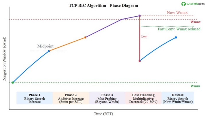
Let's now understand the working of TCP BIC algorithm in its various phases −
Binary Search Increase Phase
When the difference between Wmax and cwnd is large, TCP BIC uses binary search to find the optimal window size. The midpoint between Wmin and Wmax is calculated, and cwnd increases toward this midpoint. This allows rapid convergence to the optimal window size.
Additive Increase Phase
When cwnd is close to Wmax, TCP BIC switches to a slow additive increase mode. The window then increases by a small amount (Smin) per RTT to probe for additional bandwidth.
Max Probing Phase
After cwnd reaches and exceeds the previous Wmax, TCP BIC enters max probing mode. It continues to increase the window using a slow additive increase to search for new maximum capacity. If no loss occurs, the new Wmax is updated.
Fast Convergence
When it experiences a loss at a window size smaller than its previous Wmax, it then reduces Wmax to release bandwidth more quickly to competing flows.
Loss Handling
In case of packet loss, TCP BIC follows the routine given below −
- Sets Wmax to the current cwnd.
- Reduces cwnd using multiplicative decrease to 70-80% of current cwnd. In previous TCP algorithms (Reno and New Reno cwnd was reduced to half).
- Sets Wmin to the reduced cwnd.
- Begins binary search between Wmin and Wmax.
Example
Here is an example demonstrating TCP BIC behavior with packet loss. Initially, cwnd = 10, Wmax = 1000, Smax = 32, Smin = 1
Initial State:
cwnd = 10, Wmax = undefined, Smax = 32, Smin = 1

RTT 1-3: Binary search increase
cwnd grows: 10 => 42 => 74

RTT 4: cwnd = 106
RTT 5: cwnd = 138, Packet loss occurs(assumed)
=> Wmax = 138
=> cwnd = 138 * 0.8 = 110 (using β = 0.8)
=> Wmin = 110

RTT 6: Binary search between Wmin=110 and Wmax=138
=> target = (110 + 138) / 2 = 124
=> cwnd = 124

RTT 7: Continue binary search
=> Distance to Wmax = 138 - 124 = 14 (< Smax=32)
=> Switch to additive increase
=> cwnd = 131

RTT 8: Additive increase continues
=> cwnd = 134

RTT 9: Approaching Wmax
=> cwnd = 136

RTT 10: Near Wmax
=> cwnd = 137

RTT 11: Reached Wmax
=> cwnd = 138

RTT 12: Max probing (cwnd >= Wmax), Packet loss occurs
=> Fast convergence applied (Wmax < prev_Wmax)
=> Wmax = 138 * (2.0 - 0.8) / 2.0 = 127
=> cwnd = 138 * 0.8 = 110
=> Wmin = 110

RTT 13: Binary search resumes
=> target = (110 + 127) / 2 = 118
=> cwnd = 118

RTT 14: Continue toward target
=> cwnd = 122
Steps to Implement TCP BIC Algorithm
Here are the steps to implement TCP BIC algorithm given below −
- Initially, set the cwnd = 1 MSS, initial value of ssthresh, the number of iterations and iteration in which packet loss will occur i.e., 5 and 12.
- In Slow Start phase increase cwnd by 1 MSS for every ACK received.
- When cwnd reaches ssthresh, switch to Binary Increase Congestion control phase.
- On packet loss, set the current cwnd as Wmax and set ssthresh = cwnd * beta (where beta = 0.8).
- Set cwnd = ssthresh and calculate the midpoint between cwnd and Wmax.
- In Binary Search Increase phase, increase cwnd to the midpoint between current cwnd and Wmax.
- If no loss occurs, continue binary search by setting new midpoint between updated cwnd and Wmax.
- When cwnd reaches close to Wmax, switch to Additive Increase phase.
- In Additive Increase phase, increase cwnd linearly by a small constant for each RTT.
- If cwnd becomes greater than previous Wmax without loss, enter Max Probing phase and increase cwnd more aggressively.
- In case of timeout, reset cwnd to 1 MSS, set Wmax = 0, and restart from Slow Start.
Code Implementation
Here is the code implementation of the above steps for TCP BIC algorithm in C++, Java, and python −
#include <iostream>
#include <algorithm>
#include <cmath>
using namespace std;

class TCPBIC {
private:
    double cwnd;
    double wmax;
    double wmin;
    int smax;
    int smin;
    double beta;
    bool fast_convergence;
    double prev_wmax;

public:
    TCPBIC(double init_cwnd = 10.0, int max_inc = 32, int min_inc = 1,
           double b = 0.8, bool fc = true) {
        cwnd = init_cwnd;
        wmax = 1000.0;
        wmin = 0.0;
        smax = max_inc;
        smin = min_inc;
        beta = b;
        fast_convergence = fc;
        prev_wmax = wmax;
    }

    void onAck() {
        double target;

        if (cwnd < wmax) {
            // Binary search increase
            target = (wmax + wmin) / 2.0;
            double diff = target - cwnd;

            if (diff > smax) {
                cwnd += smax;
            } else if (diff > smin) {
                cwnd += diff / 2.0;
            } else {
                cwnd += smin;
            }
        } else {
            // Max probing - slow additive increase
            cwnd += smin;
            wmax = cwnd;
        }
    }

    void onLoss() {
        // Fast convergence check
        if (fast_convergence && wmax < prev_wmax) {
            prev_wmax = wmax;
            wmax = wmax * (2.0 - beta) / 2.0;
        } else {
            prev_wmax = wmax;
        }

        wmax = cwnd;
        cwnd = cwnd * beta;
        wmin = cwnd;
    }

    double getCwnd() { return cwnd; }
    double getWmax() { return wmax; }

    void printState(int rtt) {
        cout << rtt << "\t" << (int)cwnd << "\t\t" << (int)wmax << endl;
    }
};

int main() {
    TCPBIC bic(10.0);
    int maxRTT = 15;
    int lossRound1 = 5;
    int lossRound2 = 12;

    cout << "RTT\tcwnd\t\tWmax" << endl;

    for (int r = 1; r <= maxRTT; r++) {
        bic.printState(r);

        if (r == lossRound1) {
            cout << "=> Packet loss detected at RTT " << r << endl;
            bic.onLoss();
            cout << "=> cwnd reduced, Wmax updated" << endl;
        } else if (r == lossRound2) {
            cout << "=> Packet loss detected at RTT " << r << endl;
            bic.onLoss();
            cout << "=> cwnd reduced, fast convergence applied" << endl;
        } else {
            bic.onAck();
        }
    }

    return 0;
}
The output of the above code is as follows −
RTT	cwnd		Wmax
1	10		1000
2	42		1000
3	74		1000
4	106		1000
5	138		1000
=> Packet loss detected at RTT 5
=> cwnd reduced, Wmax updated
6	110		138
7	124		138
8	131		138
9	134		138
10	136		138
11	137		138
12	138		138
=> Packet loss detected at RTT 12
=> cwnd reduced, fast convergence applied
13	110		127
14	118		127
15	122		127
class TCPBIC {
    private double cwnd;
    private double wmax;
    private double wmin;
    private int smax;
    private int smin;
    private double beta;
    private boolean fastConvergence;
    private double prevWmax;

    public TCPBIC(double initCwnd, int maxInc, int minInc,
                  double b, boolean fc) {
        this.cwnd = initCwnd;
        this.wmax = 1000.0;
        this.wmin = 0.0;
        this.smax = maxInc;
        this.smin = minInc;
        this.beta = b;
        this.fastConvergence = fc;
        this.prevWmax = wmax;
    }

    public void onAck() {
        double target;

        if (cwnd < wmax) {
            // Binary search increase
            target = (wmax + wmin) / 2.0;
            double diff = target - cwnd;

            if (diff > smax) {
                cwnd += smax;
            } else if (diff > smin) {
                cwnd += diff / 2.0;
            } else {
                cwnd += smin;
            }
        } else {
            // Max probing
            cwnd += smin;
            wmax = cwnd;
        }
    }

    public void onLoss() {
        // Fast convergence check
        if (fastConvergence && wmax < prevWmax) {
            prevWmax = wmax;
            wmax = wmax * (2.0 - beta) / 2.0;
        } else {
            prevWmax = wmax;
        }

        wmax = cwnd;
        cwnd = cwnd * beta;
        wmin = cwnd;
    }

    public double getCwnd() { return cwnd; }
    public double getWmax() { return wmax; }

    public void printState(int rtt) {
        System.out.println(rtt + "\t" + (int)cwnd + "\t\t" + (int)wmax);
    }
}

public class Main {
    public static void main(String[] args) {
        TCPBIC bic = new TCPBIC(10.0, 32, 1, 0.8, true);
        int maxRTT = 15;
        int lossRound1 = 5;
        int lossRound2 = 12;

        System.out.println("RTT\tcwnd\t\tWmax");

        for (int r = 1; r <= maxRTT; r++) {
            bic.printState(r);

            if (r == lossRound1) {
                System.out.println("=> Packet loss detected at RTT " + r);
                bic.onLoss();
                System.out.println("=> cwnd reduced, Wmax updated");
            } else if (r == lossRound2) {
                System.out.println("=> Packet loss detected at RTT " + r);
                bic.onLoss();
                System.out.println("=> cwnd reduced, fast convergence applied");
            } else {
                bic.onAck();
            }
        }
    }
}
The output of the above code is as follows −
RTT	cwnd		Wmax
1	10		1000
2	42		1000
3	74		1000
4	106		1000
5	138		1000
=> Packet loss detected at RTT 5
=> cwnd reduced, Wmax updated
6	110		138
7	124		138
8	131		138
9	134		138
10	136		138
11	137		138
12	138		138
=> Packet loss detected at RTT 12
=> cwnd reduced, fast convergence applied
13	110		127
14	118		127
15	122		127
class TCPBIC:
    def __init__(self, init_cwnd=10.0, max_inc=32, min_inc=1,
                 beta=0.8, fast_conv=True):
        self.cwnd = init_cwnd
        self.wmax = 1000.0
        self.wmin = 0.0
        self.smax = max_inc
        self.smin = min_inc
        self.beta = beta
        self.fast_convergence = fast_conv
        self.prev_wmax = self.wmax

    def on_ack(self):
        if self.cwnd < self.wmax:
            # Binary search increase
            target = (self.wmax + self.wmin) / 2.0
            diff = target - self.cwnd

            if diff > self.smax:
                self.cwnd += self.smax
            elif diff > self.smin:
                self.cwnd += diff / 2.0
            else:
                self.cwnd += self.smin
        else:
            # Max probing
            self.cwnd += self.smin
            self.wmax = self.cwnd

    def on_loss(self):
        # Fast convergence check
        if self.fast_convergence and self.wmax < self.prev_wmax:
            self.prev_wmax = self.wmax
            self.wmax = self.wmax * (2.0 - self.beta) / 2.0
        else:
            self.prev_wmax = self.wmax

        self.wmax = self.cwnd
        self.cwnd = self.cwnd * self.beta
        self.wmin = self.cwnd

    def print_state(self, rtt):
        print(f"{rtt}\t{int(self.cwnd)}\t\t{int(self.wmax)}")

def simulate():
    bic = TCPBIC(init_cwnd=10.0)
    max_rtt = 15
    loss_round1 = 5
    loss_round2 = 12

    print("RTT\tcwnd\t\tWmax")

    for r in range(1, max_rtt + 1):
        bic.print_state(r)

        if r == loss_round1:
            print(f"=> Packet loss detected at RTT {r}")
            bic.on_loss()
            print("=> cwnd reduced, Wmax updated")
        elif r == loss_round2:
            print(f"=> Packet loss detected at RTT {r}")
            bic.on_loss()
            print("=> cwnd reduced, fast convergence applied")
        else:
            bic.on_ack()

if __name__ == "__main__":
    simulate()
The output of the above code is as follows −
RTT	cwnd		Wmax
1	10		1000
2	42		1000
3	74		1000
4	106		1000
5	138		1000
=> Packet loss detected at RTT 5
=> cwnd reduced, Wmax updated
6	110		138
7	124		138
8	131		138
9	134		138
10	136		138
11	137		138
12	138		138
=> Packet loss detected at RTT 12
=> cwnd reduced, fast convergence applied
13	110		127
14	118		127
15	122		127
Pros and Cons of TCP BIC Algorithm
The advantages of TCP BIC algorithm are listed below −
- Better scalability in high bandwidth-delay product networks.
- Fast convergence to optimal window size with binary search.
- Less aggressive multiplicative decrease. This results in saving more bandwidth.
- Additive increase provides stability near optimal window size.
Here are the limitations of TCP BIC algorithm −
- It can cause excessive packet loss.
- Complex implementation than traditional TCP algorithms.
Difference between TCP Reno and TCP BIC Algorithm
The follwing table highlights the major differences between TCP Reno and TCP BIC algorithm −
| TCP Reno Algorithm | TCP BIC Algorithm |
|---|---|
| It uses AIMD with linear growth. | It uses binary search increase with both quick and slow phases. |
| It is simple to implement. | It is more complex to implement. |
| It reduces cwnd to 50% on packet loss. | It reduces cwnd to 80% on packet loss. |
| Scalability in high-speed networks is low. | Better scalability for high-speed networks. |
| It does not have fast convergence mechanism. | It has fast convergence mechanism. |
Conclusion
TCP BIC congestion control algorithm uses binary search to quickly move towards the optimal window size and then switch to additive increase on reaching near the optimal point. It addresses the limitations of previous TCP congestion control algorithms like Reno and New Reno.
