- Bokeh - Home
- Bokeh - Introduction
- Bokeh - Environment Setup
- Bokeh - Getting Started
- Bokeh - Jupyter Notebook
- Bokeh - Basic Concepts
- Bokeh - Plots with Glyphs
- Bokeh - Area Plots
- Bokeh - Circle Glyphs
- Bokeh - Rectangle, Oval and Polygon
- Bokeh - Wedges and Arcs
- Bokeh - Specialized Curves
- Bokeh - Setting Ranges
- Bokeh - Axes
- Bokeh - Annotations and Legends
- Bokeh - Pandas
- Bokeh - ColumnDataSource
- Bokeh - Filtering Data
- Bokeh - Layouts
- Bokeh - Plot Tools
- Bokeh - Styling Visual Attributes
- Bokeh - Customising legends
- Bokeh - Adding Widgets
- Bokeh - Server
- Bokeh - Using Bokeh Subcommands
- Bokeh - Exporting Plots
- Bokeh - Embedding Plots and Apps
- Bokeh - Extending Bokeh
- Bokeh - WebGL
- Bokeh - Developing with JavaScript
Bokeh Resources
Bokeh - Layouts
Bokeh visualizations can be suitably arranged in different layout options. These layouts as well as sizing modes result in plots and widgets resizing automatically as per the size of browser window. For consistent appearance, all items in a layout must have same sizing mode. The widgets (buttons, menus, etc.) are kept in a separate widget box and not in plot figure.
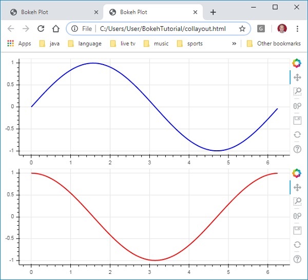
First type of layout is Column layout which displays plot figures vertically. The column() function is defined in bokeh.layouts module and takes following signature −
from bokeh.layouts import column
col = column(children, sizing_mode)
children − List of plots and/or widgets.
sizing_mode − determines how items in the layout resize. Possible values are "fixed", "stretch_both", "scale_width", "scale_height", "scale_both". Default is fixed.
Example - Displaying Figures Vertically
Following code produces two Bokeh figures and places them in a column layout so that they are displayed vertically. Line glyphs representing sine and cos relationship between x and y data series is displayed in Each figure.
main.py
from bokeh.plotting import figure, output_file, show
from bokeh.layouts import column
import numpy as np
import math

x = np.arange(0, math.pi*2, 0.05)
y1 = np.sin(x)
y2 = np.cos(x)
fig1 = figure(width = 200, height = 200)
fig1.line(x, y1,line_width = 2, line_color = 'blue')
fig2 = figure(width = 200, height = 200)
fig2.line(x, y2,line_width = 2, line_color = 'red')

c = column(children = [fig1, fig2], sizing_mode = 'stretch_both')
show(c)
Output
Run the code and verify the output in the browser.
(myenv) D:\bokeh\myenv>py main.py
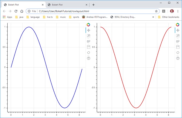
Example - Displaying Figures horizontally
Similarly, Row layout arranges plots horizontally, for which row() function as defined in bokeh.layouts module is used. As you would think, it also takes two arguments (similar to column() function) children and sizing_mode.
The sine and cos curves as shown vertically in above diagram are now displayed horizontally in row layout with following code
main.py
from bokeh.plotting import figure, output_file, show
from bokeh.layouts import row
import numpy as np
import math

x = np.arange(0, math.pi*2, 0.05)
y1 = np.sin(x)
y2 = np.cos(x)
fig1 = figure(width = 200, height = 200)
fig1.line(x, y1,line_width = 2, line_color = 'blue')
fig2 = figure(width = 200, height = 200)
fig2.line(x, y2,line_width = 2, line_color = 'red')
r = row(children = [fig1, fig2], sizing_mode = 'stretch_both')
show(r)
Output
Run the code and verify the output in the browser.
(myenv) D:\bokeh\myenv>py main.py
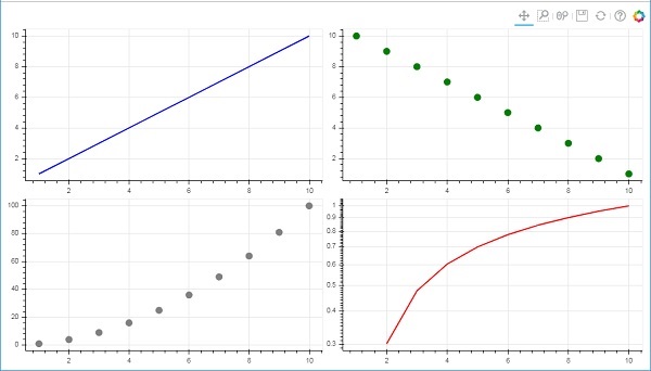
Example - Grid Layout
The Bokeh package also has grid layout. It holds multiple plot figures (as well as widgets) in a two dimensional grid of rows and columns. The gridplot() function in bokeh.layouts module returns a grid and a single unified toolbar which may be positioned with the help of toolbar_location property.
This is unlike row or column layout where each plot shows its own toolbar. The grid() function too uses children and sizing_mode parameters where children is a list of lists. Ensure that each sublist is of same dimensions.
In the following code, four different relationships between x and y data series are plotted in a grid of two rows and two columns.
main.py
from bokeh.plotting import figure, output_file, show
from bokeh.layouts import gridplot
import math
x = list(range(1,11))

y1 = x
y2 =[11-i for i in x]
y3 = [i*i for i in x]
y4 = [math.log10(i) for i in x]

fig1 = figure(width = 200, height = 200)
fig1.line(x, y1,line_width = 2, line_color = 'blue')
fig2 = figure(width = 200, height = 200)
fig2.scatter(x, y2,size = 10, color = 'green')
fig3 = figure(width = 200, height = 200)
fig3.scatter(x,y3, size = 10, color = 'grey')
fig4 = figure(width = 200, height = 200, y_axis_type = 'log')
fig4.line(x,y4, line_width = 2, line_color = 'red')
grid = gridplot(children = [[fig1, fig2], [fig3,fig4]], sizing_mode = 'stretch_both')
show(grid)
Output
Run the code and verify the output in the browser.
(myenv) D:\bokeh\myenv>py main.py