- Bokeh - Home
- Bokeh - Introduction
- Bokeh - Environment Setup
- Bokeh - Getting Started
- Bokeh - Jupyter Notebook
- Bokeh - Basic Concepts
- Bokeh - Plots with Glyphs
- Bokeh - Area Plots
- Bokeh - Circle Glyphs
- Bokeh - Rectangle, Oval and Polygon
- Bokeh - Wedges and Arcs
- Bokeh - Specialized Curves
- Bokeh - Setting Ranges
- Bokeh - Axes
- Bokeh - Annotations and Legends
- Bokeh - Pandas
- Bokeh - ColumnDataSource
- Bokeh - Filtering Data
- Bokeh - Layouts
- Bokeh - Plot Tools
- Bokeh - Styling Visual Attributes
- Bokeh - Customising legends
- Bokeh - Adding Widgets
- Bokeh - Server
- Bokeh - Using Bokeh Subcommands
- Bokeh - Exporting Plots
- Bokeh - Embedding Plots and Apps
- Bokeh - Extending Bokeh
- Bokeh - WebGL
- Bokeh - Developing with JavaScript
Bokeh Resources
Bokeh - Filtering Data
Often, you may want to obtain a plot pertaining to a part of data that satisfies certain conditions instead of the entire dataset. Object of the CDSView class defined in bokeh.models module returns a subset of ColumnDatasource under consideration by applying one or more filters over it.
IndexFilter is the simplest type of filter. You have to specify indices of only those rows from the dataset that you want to use while plotting the figure.
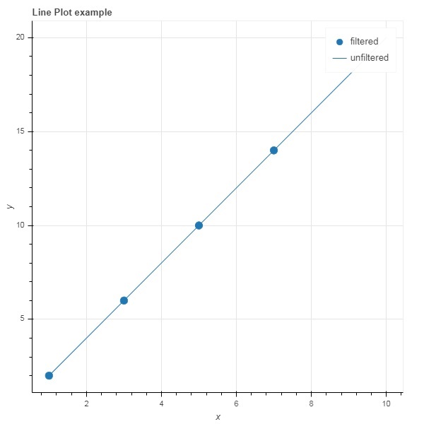
Following example demonstrates use of IndexFilter to set up a CDSView. The resultant figure shows a line glyph between x and y data series of the ColumnDataSource. A view object is obtained by applying index filter over it. The view is used to plot circle glyph as a result of IndexFilter.
Example - Usage of IndexFilter
main.py
from bokeh.models import ColumnDataSource, CDSView, IndexFilter
from bokeh.plotting import figure, output_file, show

source = ColumnDataSource(data = dict(x = list(range(1,11)), y = list(range(2,22,2))))
view = CDSView(filter = IndexFilter([0, 2, 4,6]))
fig = figure(title = 'Line Plot example', x_axis_label = 'x', y_axis_label = 'y')
fig.scatter(x = "x", y = "y", size = 10, source = source, view = view, legend_label = 'filtered')
fig.line(source.data['x'],source.data['y'], legend_label = 'unfiltered')
show(fig)
Output
Run the code and verify the output in the browser.
(myenv) D:\bokeh\myenv>py main.py
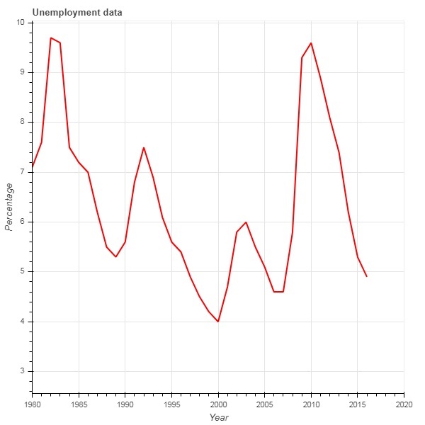
Example - Usage of BooleanFilter
To choose only those rows from the data source, that satisfy a certain Boolean condition, apply a BooleanFilter.
A typical Bokeh installation consists of a number of sample data sets in sampledata directory. For following example, we use unemployment1948 dataset provided in the form of unemployment1948.csv. It stores year wise percentage of unemployment in USA since 1948. We want to generate a plot only for year 1980 onwards. For that purpose, a CDSView object is obtained by applying BooleanFilter over the given data source.
main.py
from bokeh.models import ColumnDataSource, CDSView, BooleanFilter
from bokeh.plotting import figure, show
from bokeh.sampledata.unemployment1948 import data

source = ColumnDataSource(data)
booleans = [True if int(year) >= 1980 else False for year in source.data['Year']]
print (booleans)
view1 = CDSView(filter=BooleanFilter(booleans))
p = figure(title = "Unemployment data", x_range = (1980,2020), x_axis_label = 'Year', y_axis_label='Percentage')
p.line(x = 'Year', y = 'Annual', source = source, view = view1, color = 'red', line_width = 2)
show(p)
Output
Run the code and verify the output in the browser.
(myenv) D:\bokeh\myenv>py main.py
Example - Usage of CustomJSFilter
To add more flexibility in applying filter, Bokeh provides a CustomJSFilter class with the help of which the data source can be filtered with a user defined JavaScript function.
The example given below uses the same USA unemployment data. Defining a CustomJSFilter to plot unemployment figures of year 1980 and after.
main.py
from bokeh.models import ColumnDataSource, CDSView, CustomJSFilter
from bokeh.plotting import figure, show
from bokeh.sampledata.unemployment1948 import data

source = ColumnDataSource(data)
custom_filter = CustomJSFilter(code = '''
   var indices = [];

   for (var i = 0; i < source.get_length(); i++){
      if (parseInt(source.data['Year'][i]) > = 1980){
         indices.push(true);
      } else {
         indices.push(false);
      }
   }
   return indices;
''')
view1 = CDSView(filter = custom_filter)
p = figure(title = "Unemployment data", x_range = (1980,2020), x_axis_label = 'Year', y_axis_label = 'Percentage')
p.line(x = 'Year', y = 'Annual', source = source, view = view1, color = 'red', line_width = 2)
show(p)
Output
Run the code and verify the output in the browser.
(myenv) D:\bokeh\myenv>py main.py
