- Bokeh - Home
- Bokeh - Introduction
- Bokeh - Environment Setup
- Bokeh - Getting Started
- Bokeh - Jupyter Notebook
- Bokeh - Basic Concepts
- Bokeh - Plots with Glyphs
- Bokeh - Area Plots
- Bokeh - Circle Glyphs
- Bokeh - Rectangle, Oval and Polygon
- Bokeh - Wedges and Arcs
- Bokeh - Specialized Curves
- Bokeh - Setting Ranges
- Bokeh - Axes
- Bokeh - Annotations and Legends
- Bokeh - Pandas
- Bokeh - ColumnDataSource
- Bokeh - Filtering Data
- Bokeh - Layouts
- Bokeh - Plot Tools
- Bokeh - Styling Visual Attributes
- Bokeh - Customising legends
- Bokeh - Adding Widgets
- Bokeh - Server
- Bokeh - Using Bokeh Subcommands
- Bokeh - Exporting Plots
- Bokeh - Embedding Plots and Apps
- Bokeh - Extending Bokeh
- Bokeh - WebGL
- Bokeh - Developing with JavaScript
Bokeh Resources
Bokeh - Axes
In this chapter, we shall discuss about various types of axes.
| Sr.No | Axes | Description |
|---|---|---|
| 1 | Categorical Axes | The bokeh plots show numerical data along both x and y axes. In order to use categorical data along either of axes, we need to specify a FactorRange to specify categorical dimensions for one of them. |
| 2 | Log Scale Axes | If there exists a power law relationship between x and y data series, it is desirable to use log scales on both axes. |
| 3 | Twin Axes | It may be needed to show multiple axes representing varying ranges on a single plot figure. The figure object can be so configured by defining extra_x_range and extra_y_range properties |
Categorical Axes
In the examples so far, the Bokeh plots show numerical data along both x and y axes. In order to use categorical data along either of axes, we need to specify a FactorRange to specify categorical dimensions for one of them. For example, to use strings in the given list for x axis −
langs = ['C', 'C++', 'Java', 'Python', 'PHP']
fig = figure(x_range = langs, plot_width = 300, plot_height = 300)
Example - Plotting a simple bar plot (main.py)
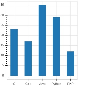
With following example, a simple bar plot is displayed showing number of students enrolled for various courses offered.
from bokeh.plotting import figure, output_file, show

langs = ['C', 'C++', 'Java', 'Python', 'PHP']
students = [23,17,35,29,12]
fig = figure(x_range = langs, width = 300, height = 300)
fig.vbar(x = langs, top = students, width = 0.5)

show(fig)
Output
Run the code and verify the output in the browser.
(myenv) D:\bokeh\myenv>py main.py
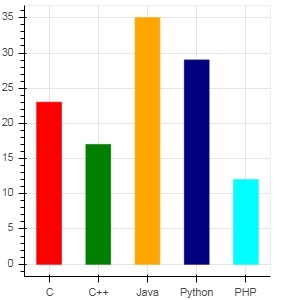
To show each bar in different colour, set color property of vbar() function to list of color values.
main.py
from bokeh.plotting import figure, output_file, show

langs = ['C', 'C++', 'Java', 'Python', 'PHP']
students = [23,17,35,29,12]
fig = figure(x_range = langs, width = 300, height = 300)

cols = ['red','green','orange','navy', 'cyan']
fig.vbar(x = langs, top = students, color = cols,width=0.5)

show(fig)
Output
Run the code and verify the output in the browser.
(myenv) D:\bokeh\myenv>py main.py
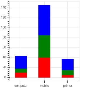
To render a vertical (or horizontal) stacked bar using vbar_stack() or hbar_stack() function, set stackers property to list of fields to stack successively and source property to a dict object containing values corresponding to each field.
In following example, sales is a dictionary showing sales figures of three products in three months.
main.py
from bokeh.plotting import figure, output_file, show

products = ['computer','mobile','printer']
months = ['Jan','Feb','Mar']
sales = {'products':products,
   'Jan':[10,40,5],
   'Feb':[8,45,10],
   'Mar':[25,60,22]}
cols = ['red','green','blue']#,'navy', 'cyan']
fig = figure(x_range = products, width = 300, height = 300)
fig.vbar_stack(months, x = 'products', source = sales, color = cols,width = 0.5)

show(fig)
Output
Run the code and verify the output in the browser.
(myenv) D:\bokeh\myenv>py main.py
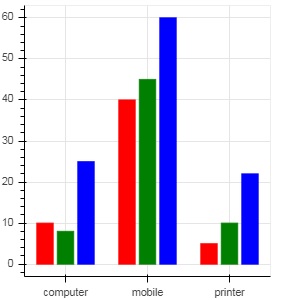
A grouped bar plot is obtained by specifying a visual displacement for the bars with the help of dodge() function in bokeh.transform module.
The dodge() function introduces a relative offset for each bar plot thereby achieving a visual impression of group. In following example, vbar() glyph is separated by an offset of 0.25 for each group of bars for a particular month.
main.py
from bokeh.plotting import figure, output_file, show
from bokeh.transform import dodge

products = ['computer','mobile','printer']
months = ['Jan','Feb','Mar']
sales = {'products':products,
   'Jan':[10,40,5],
   'Feb':[8,45,10],
   'Mar':[25,60,22]}
fig = figure(x_range = products, width = 300, height = 300)
fig.vbar(x = dodge('products', -0.25, range = fig.x_range), top = 'Jan',
   width = 0.2,source = sales, color = "red")
fig.vbar(x = dodge('products', 0.0, range = fig.x_range), top = 'Feb',
   width = 0.2, source = sales,color = "green")
fig.vbar(x = dodge('products', 0.25, range = fig.x_range), top = 'Mar',
   width = 0.2,source = sales,color = "blue")

show(fig)
Output
Run the code and verify the output in the browser.
(myenv) D:\bokeh\myenv>py main.py
Log Scale Axes
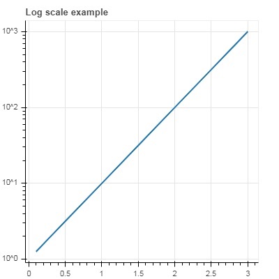
When values on one of the axes of a plot grow exponentially with linearly increasing values of another, it is often necessary to have the data on former axis be displayed on a log scale. For example, if there exists a power law relationship between x and y data series, it is desirable to use log scales on both axes.
Bokeh.plotting API's figure() function accepts x_axis_type and y_axis_type as arguments which may be specified as log axis by passing "log" for the value of either of these parameters.
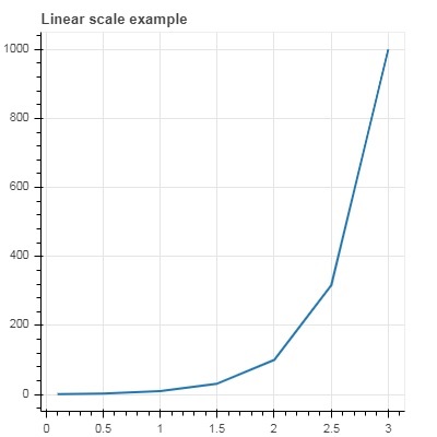
First figure shows plot between x and 10x on a linear scale. In second figure y_axis_type is set to 'log'
main.py
from bokeh.plotting import figure, output_file, show

x = [0.1, 0.5, 1.0, 1.5, 2.0, 2.5, 3.0]
y = [10**i for i in x]
fig = figure(title = 'Linear scale example',width = 400, height = 400)
fig.line(x, y, line_width = 2)

show(fig)
Output
Run the code and verify the output in the browser.
(myenv) D:\bokeh\myenv>py main.py
Now change figure() function to configure y_axis_type=log
main.py
from bokeh.plotting import figure, output_file, show

x = [0.1, 0.5, 1.0, 1.5, 2.0, 2.5, 3.0]
y = [10**i for i in x]
fig = figure(title = 'Linear scale example',width = 400, height = 400, y_axis_type = "log")
fig.line(x, y, line_width = 2)

show(fig)
Output
Run the code and verify the output in the browser.
(myenv) D:\bokeh\myenv>py main.py
Twin Axes
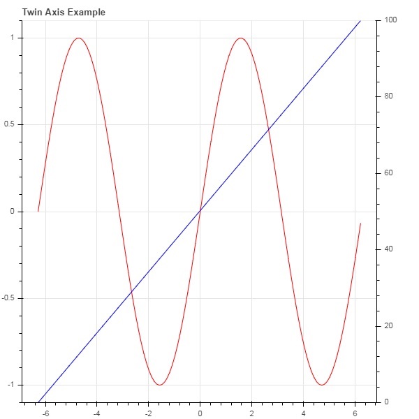
In certain situations, it may be needed to show multiple axes representing varying ranges on a single plot figure. The figure object can be so configured by defining extra_x_range and extra_y_range properties. While adding new glyph to the figure, these named ranges are used.
We try to display a sine curve and a straight line in same plot. Both glyphs have y axes with different ranges. The x and y data series for sine curve and line are obtained by the following −
from numpy import pi, arange, sin, linspace
x = arange(-2*pi, 2*pi, 0.1)
y = sin(x)
y2 = linspace(0, 100, len(y))
Here, plot between x and y represents sine relation and plot between x and y2 is a straight line. The Figure object is defined with explicit y_range and a line glyph representing sine curve is added as follows −
fig = figure(title = 'Twin Axis Example', y_range = (-1.1, 1.1))
fig.line(x, y, color = "red")
We need an extra y range. It is defined as −
fig.extra_y_ranges = {"y2": Range1d(start = 0, end = 100)}
To add additional y axis on right side, use add_layout() method. Add a new line glyph representing x and y2 to the figure.
fig.add_layout(LinearAxis(y_range_name = "y2"), 'right')
fig.line(x, y2, color = "blue", y_range_name = "y2")
This will result in a plot with twin y axes. Complete code and the output is as follows −
from numpy import pi, arange, sin, linspace
x = arange(-2*pi, 2*pi, 0.1)
y = sin(x)
y2 = linspace(0, 100, len(y))
from bokeh.plotting import output_file, figure, show
from bokeh.models import LinearAxis, Range1d
fig = figure(title='Twin Axis Example', y_range = (-1.1, 1.1))
fig.line(x, y, color = "red")
fig.extra_y_ranges = {"y2": Range1d(start = 0, end = 100)}
fig.add_layout(LinearAxis(y_range_name = "y2"), 'right')
fig.line(x, y2, color = "blue", y_range_name = "y2")
show(fig)
Output
Run the code and verify the output in the browser.
(myenv) D:\bokeh\myenv>py main.py