Importing Data into Excel

---

---

You might have to use data from various sources for analysis. In Excel, you can import data from different data sources. Some of the data sources are as follows −

• Microsoft Access Database
• Web Page
• Text File
• SQL Server Table
• SQL Server Analysis Cube
• XML File

You can import any number of tables simultaneously from a database.

Importing Data from Microsoft Access Database

We will learn how to import data from MS Access database. Follow the steps given below −

Step 1 − Open a new blank workbook in Excel.

Step 2 − Click the DATA tab on the Ribbon.

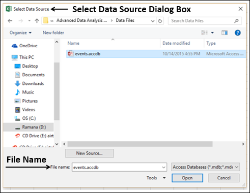
Step 3 − Click From Access in the Get External Data group. The Select Data Source dialog box appears.

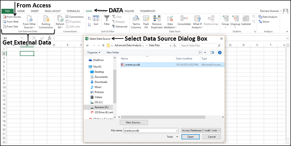
Step 4 − Select the Access database file that you want to import. Access database files will have the extension .accdb.

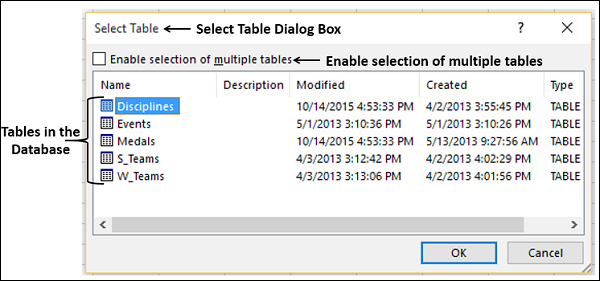
The Select Table dialog box appears displaying the tables found in the Access database. You can either import all the tables in the database at once or import only the selected tables based on your data analysis needs.

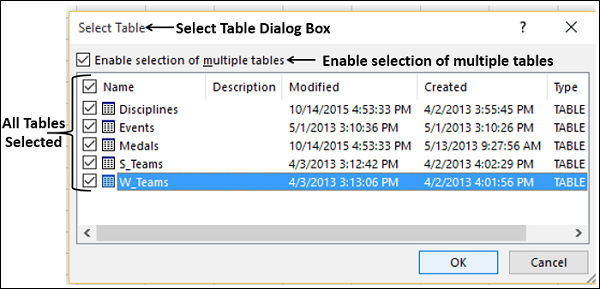
Step 5 − Select the Enable selection of multiple tables box and select all the tables.

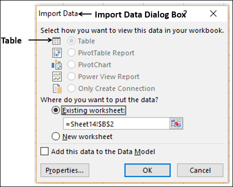
Step 6 − Click OK. The Import Data dialog box appears.

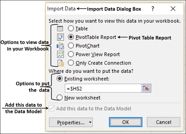
As you observe, you have the following options to view the data you are importing in your workbook −

• Table
• PivotTable Report
• PivotChart
• Power View Report

You also have an option - only create connection. Further, PivotTable Report is selected by default.

Excel also gives you the options to put the data in your workbook −

• Existing worksheet
• New worksheet

You will find another check box that is selected and disabled – Add this data to the Data Model. Whenever you import data tables into your workbook, they are automatically added to the Data Model in your workbook. You will learn more about the Data Model in later chapters.

You can try each one of the options to view the data you are importing, and check how the data appears in your workbook −

• If you select Table, Existing worksheet option gets disabled, New worksheet option gets selected and Excel creates as many worksheets as the number of tables you are importing from the database. The Excel tables appear in these worksheets.

• If you select PivotTable Report, Excel imports the tables into the workbook and creates an empty PivotTable for analyzing the data in the imported tables. You have an option to create the PivotTable in an existing worksheet or a new worksheet.

  Excel tables for the imported data tables will not appear in the workbook. However, you will find all the data tables in the PivotTable fields list, along with the fields in each table.

• If you select PivotChart, Excel imports the tables into the workbook and creates an empty PivotChart for displaying the data in the imported tables. You have an option to create the PivotChart in an existing worksheet or a new worksheet.

  Excel tables for the imported data tables will not appear in the workbook. However, you will find all the data tables in the PivotChart fields list, along with the fields in each table.

• If you select Power View Report, Excel imports the tables into the workbook and creates a Power View Report in a new worksheet. You will learn how to use Power View Reports for analyzing data in later chapters.

  Excel tables for the imported data tables will not appear in the workbook. However, you will find all the data tables in the Power View Report fields list, along with the fields in each table.

• If you select the option - Only Create Connection, a data connection will be established between the database and your workbook. No tables or reports appear in the workbook. However, the imported tables are added to the Data Model in your workbook by default.

  You need to choose any of these options, based on your intent of importing data for data analysis. As you observed above, irrespective of the option you have chosen, the data is imported and added to the Data Model in your workbook.

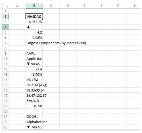
Importing Data from a Web Page

Sometimes, you might have to use the data that is refreshed on a web site. You can import data from a table on a website into Excel.

Step 1 − Open a new blank workbook in Excel.

Step 2 − Click the DATA tab on the Ribbon.

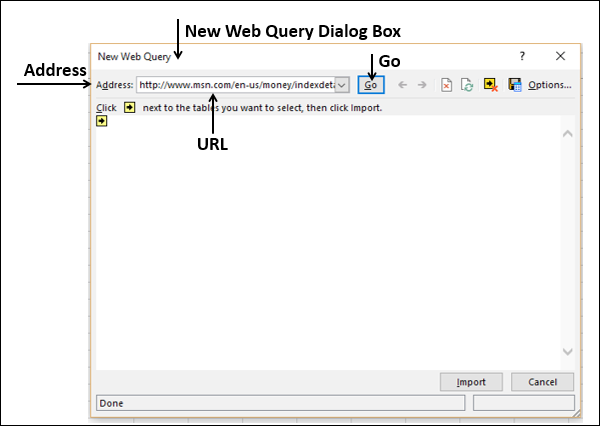
Step 3 − Click From Web in the Get External Data group. The New Web Query dialog box appears.

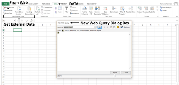
Step 4 − Enter the URL of the web site from where you want to import data, in the box next to Address and click Go.

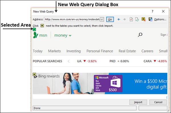
Step 5 − The data on the website appears. There will be yellow arrow icons next to the table data that can be imported.

Step 6 − Click the yellow icons to select the data you want to import. This turns the yellow icons to green boxes with a checkmark as shown in the following screen shot.

Step 7 − Click the Import button after you have selected what you want.

The Import Data dialog box appears.

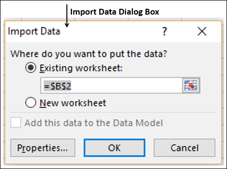
Step 8 − Specify where you want to put the data and click Ok.

Step 9 − Arrange the data for further analysis and/or presentation.

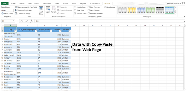
Copy-pasting data from web

Another way of getting data from a web page is by copying and pasting the required data.

Step 1 − Insert a new worksheet.

Step 2 − Copy the data from the web page and paste it on the worksheet.

Step 3 − Create a table with the pasted data.

Importing Data from a Text File

If you have data in .txt or .csv or .prn files, you can import data from those files treating them as text files. Follow the steps given below −

Step 1 − Open a new worksheet in Excel.

Step 2 − Click the DATA tab on the Ribbon.

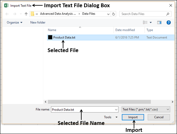
Step 3 − Click From Text in the Get External Data group. The Import Text File dialog box appears.

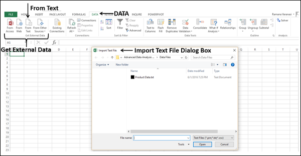
You can see that .prn, .txt and .csv extension text files are accepted.

Step 4 − Select the file. The selected file name appears in the File name box. The Open button changes to Import button.

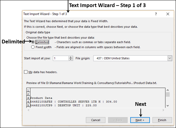
Step 5 − Click the Import button. Text Import Wizard – Step 1 of 3 dialog box appears.

Step 6 − Click the option Delimited to choose the file type and click Next.

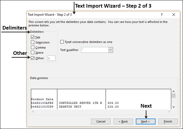
The Text Import Wizard – Step 2 of 3 dialog box appears.

Step 7 − Under Delimiters, select Other.

Step 8 − In the box next to Other, type | (That is the delimiter in the text file you are importing).

Step 9 − Click Next.

The Text Import Wizard – Step 3 of 3 dialog box appears.

Step 10 − In this dialog box, you can set column data format for each of the columns.

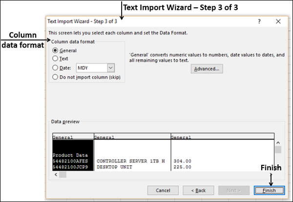
Step 11 − After you complete the data formatting of columns, click Finish. The Import Data dialog box appears.

You will observe the following −

• Table is selected for view and is grayed. Table is the only view option you have in this case.

• You can put the data either in an existing worksheet or a New worksheet.

• You can select or not select the check box Add this data to the Data Model.

• Click OK after you have made the choices.

Data appears on the worksheet you specified. You have imported data from Text file into Excel workbook.

Importing Data from another Workbook

You might have to use data from another Excel workbook for your data analysis, but someone else might maintain the other workbook.

To get up to date data from another workbook, establish a data connection with that workbook.

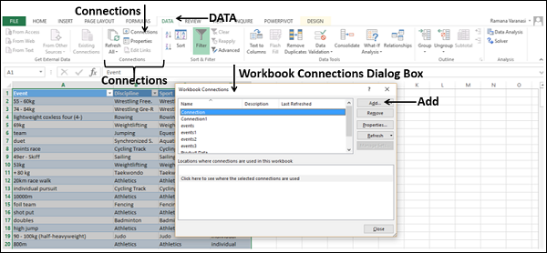
Step 1 − Click DATA > Connections in the Connections group on the Ribbon.

The Workbook Connections dialog box appears.

Step 2 − Click the Add button in the Workbook Connections dialog box. The Existing Connections dialog box appears.

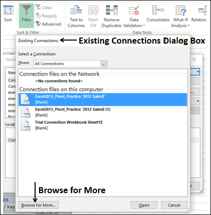
Step 3 − Click Browse for More… button. The Select Data Source dialog box appears.

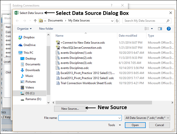
Step 4 − Click the New Source button. The Data Connection Wizard dialog box appears.

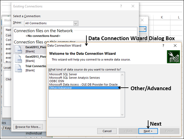
Step 5 − Select Other/Advanced in the data source list and click Next. The Data Link Properties dialog box appears.

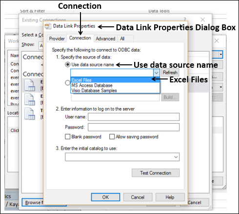
Step 6 − Set the data link properties as follows −

• Click the Connection tab.

• Click Use data source name.

• Click the down-arrow and select Excel Files from the drop-down list.

• Click OK.

The Select Workbook dialog box appears.

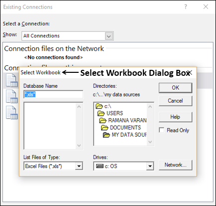
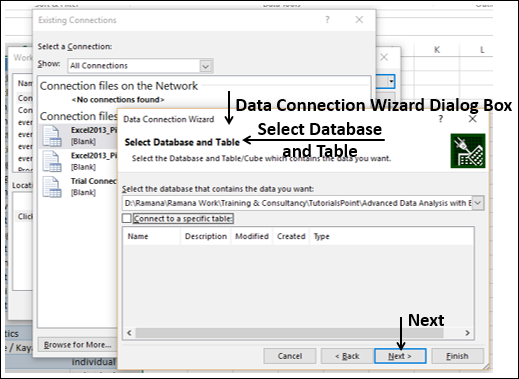
Step 7 − Browse to the location where you have the workbook to be imported is located. Click OK.

The Data Connection Wizard dialog box appears with Select Database and Table.

Note − In this case, Excel treats each worksheet that is getting imported as a table. The table name will be the worksheet name. So, to have meaningful table names, name / rename the worksheets as appropriate.

Step 8 − Click Next. The Data Connection Wizard dialog box appears with Save Data Connection File and Finish.

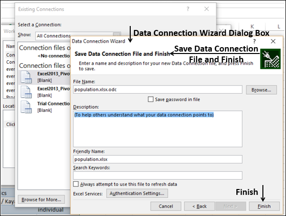
Step 9 − Click the Finish button. The Select Table dialog box appears.

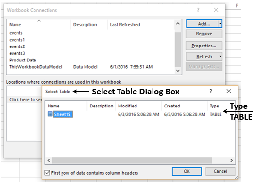
As you observe, Name is the worksheet name that is imported as type TABLE. Click OK.

The Data connection with the workbook you have chosen will be established.

Importing Data from Other Sources

Excel provides you options to choose various other data sources. You can import data from these in few steps.

Step 1 − Open a new blank workbook in Excel.

Step 2 − Click the DATA tab on the Ribbon.

Step 3 − Click From Other Sources in the Get External Data group.

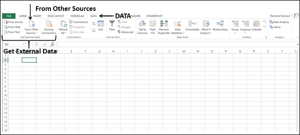
Dropdown with various data sources appears.

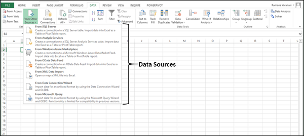
You can import data from any of these data sources into Excel.

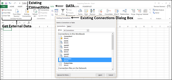
Importing Data using an Existing Connection

In an earlier section, you have established a data connection with a workbook.

Now, you can import data using that existing connection.

Step 1 − Click the DATA tab on the Ribbon.

Step 2 − Click Existing Connections in the Get External Data group. The Existing Connections dialog box appears.

Step 3 − Select the connection from where you want to import data and click Open.

Renaming the Data Connections

It will be useful if the data connections you have in your workbook have meaningful names for the ease of understanding and locating.

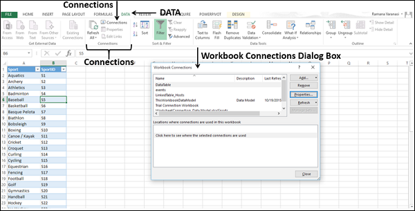
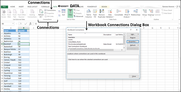
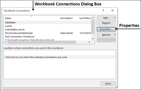
Step 1 − Go to DATA > Connections on the Ribbon. The Workbook Connections dialog box appears.

Step 2 − Select the connection that you want to rename and click Properties.

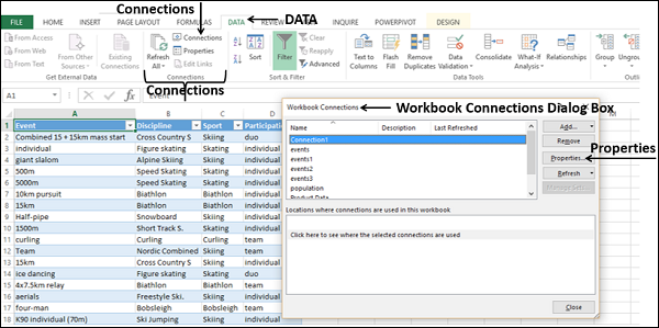
The Connection Properties dialog box appears. The present name appears in the Connection name box −

Step 3 − Edit the Connection name and click OK. The data connection will have the new name that you have given.

Refreshing an External Data Connection

When you connect your Excel workbook to an external data source, as you have seen in the above sections, you would like to keep the data in your workbook up to date reflecting the changes made to the external data source time to time.

You can do this by refreshing the data connections you have made to those data sources. Whenever you refresh the data connection, you see the most recent data changes from that data source, including anything that is new or that is modified or that has been deleted.

You can either refresh only the selected data or all the data connections in the workbook at once.

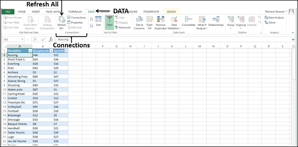
Step 1 − Click the DATA tab on the Ribbon.

Step 2 − Click Refresh All in the Connections group.

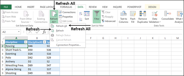
As you observe, there are two commands in the dropdown list – Refresh and Refresh All.

• If you click Refresh, the selected data in your workbook is updated.

• If you click Refresh All, all the data connections to your workbook are updated.

Updating all the Data Connections in the Workbook

You might have several data connections to your workbook. You need to update them from time to time so that your workbook will have access to the most recent data.

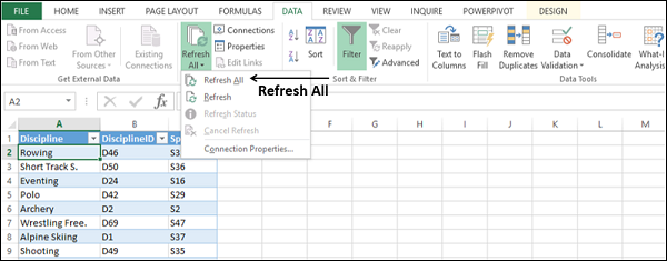
Step 1 − Click any cell in the table that contains the link to the imported data file.

Step 2 − Click the Data tab on the Ribbon.

Step 3 − Click Refresh All in the Connections group.

Step 4 − Select Refresh All from the dropdown list. All the data connections in the workbook will be updated.

Automatically Refresh Data when a Workbook is opened

You might want to have access to the recent data from the data connections to your workbook whenever your workbook is opened.

Step 1 − Click any cell in the table that contains the link to the imported data file.

Step 2 − Click the Data tab.

Step 3 − Click Connections in the Connections group.

The Workbook Connections dialog box appears.

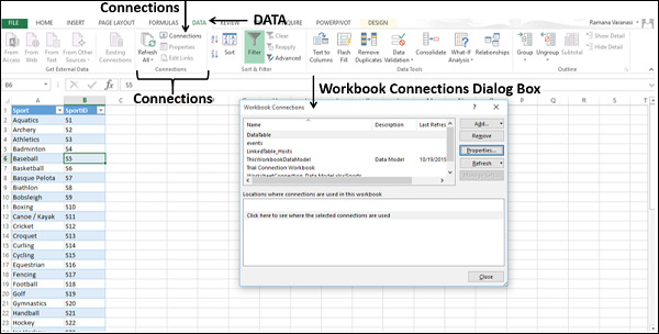
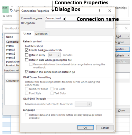
Step 4 − Click the Properties button. The Connection Properties dialog box appears.

Step 5 − Click the Usage tab.

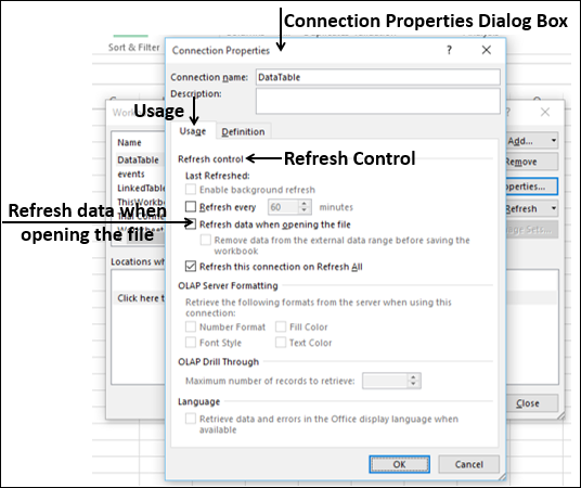
Step 6 − Check the option - Refresh data when opening the file.

You have another option also - Remove data from the external data range before saving the workbook. You can use this option to save the workbook with the query definition but without the external data.

Step 7 − Click OK. Whenever you open your workbook, the up to date data will be loaded into your workbook.

Automatically Refresh Data at regular Intervals

You might be using your workbook keeping it open for longer durations. In such a case, you might want to have the data refreshed periodically without any intervention from you.

Step 1 − Click any cell in the table that contains the link to the imported data file.

Step 2 − Click the Data tab on the Ribbon.

Step 3 − Click Connections in the Connections group.

The Workbook Connections dialog box appears.

Step 4 − Click the Properties button.

The Connection Properties dialog box appears. Set the properties as follows −

• Click the Usage tab.

• Check the option Refresh every.

• Enter 60 as the number of minutes between each refresh operation and click Ok.

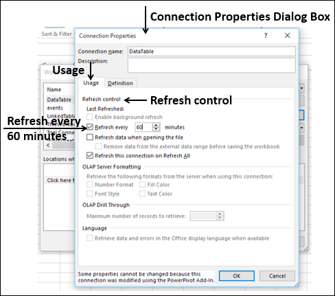
Your Data will be automatically refreshed every 60 min. (i.e. every one hour).

Enabling Background Refresh

For very large data sets, consider running a background refresh. This returns control of Excel to you instead of making you wait several minutes or more for the refresh to finish. You can use this option when you are running a query in the background. However, during this time, you cannot run a query for any connection type that retrieves data for the Data Model.

• Click in any cell in the table that contains the link to the imported data file.

• Click the Data tab.

• Click Connections in the Connections group. The Workbook Connections dialog box appears.

Click the Properties button.

The Connection Properties dialog box appears. Click the Usage tab. The Refresh Control options appear.

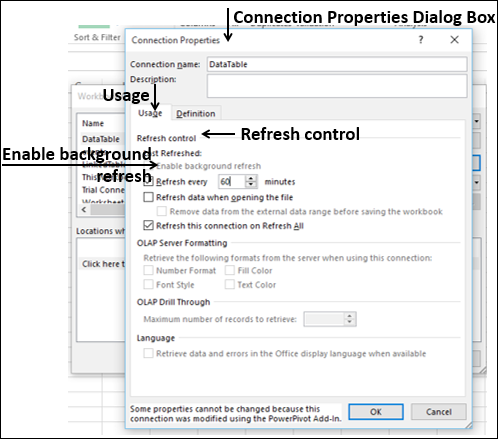
• Click Enable background refresh.
• Click OK. The Background refresh is enabled for your workbook.