- Excel Data Analysis Tutorial
- Excel Data Analysis - Home
- Data Analysis - Overview
- Data Analysis - Process
- Excel Data Analysis - Overview
- Working with Range Names
- Tables
- Cleaning Data with Text Functions
- Cleaning Data Contains Date Values
- Working with Time Values
- Conditional Formatting
- Sorting
- Filtering
- Subtotals with Ranges
- Quick Analysis
- Lookup Functions
- PivotTables
- Data Visualization
- Data Validation
- Financial Analysis
- Working with Multiple Sheets
- Formula Auditing
- Inquire
- Advanced Data Analysis
- Advanced Data Analysis - Overview
- Data Consolidation
- What-If Analysis
- What-If Analysis with Data Tables
- What-If Analysis Scenario Manager
- What-If Analysis with Goal Seek
- Optimization with Excel Solver
- Importing Data into Excel
- Data Model
- Exploring Data with PivotTables
- Exploring Data with Powerpivot
- Exploring Data with Power View
- Exploring Data Power View Charts
- Exploring Data Power View Maps
- Exploring Data PowerView Multiples
- Exploring Data Power View Tiles
- Exploring Data with Hierarchies
- Aesthetic Power View Reports
- Key Performance Indicators
- Excel Data Analysis Resources
- Excel Data Analysis - Quick Guide
- Excel Data Analysis - Resources
- Excel Data Analysis - Discussion
Advanced Data Analysis - Data Consolidation
You might have come across different situations wherein you have to present consolidated data. The source of the data could be from one place, or several places. Another challenge could be that the data might be updated by other people from time to time.
You need to know how you can set up a summary worksheet that consolidates the data from the sources that you set up, whenever you want. In Excel, you can easily perform this task in a few steps with the Data Tool – Consolidate.
Preparing Data for Consolidation
Before you begin consolidating the data, make sure that there is consistency across the data sources. This means that the data is arranged as follows −
Each range of data is on a separate worksheet.
Each range of data is in list format, with labels in the first row.
Additionally, you can have labels for the categories, if applicable, in the first column.
All the ranges of data have the same layout.
All the ranges of data contain similar facts.
There are no blank rows or columns within each range.
In case the data sources are external, ensure usage of a predefined layout in the form of an Excel template.
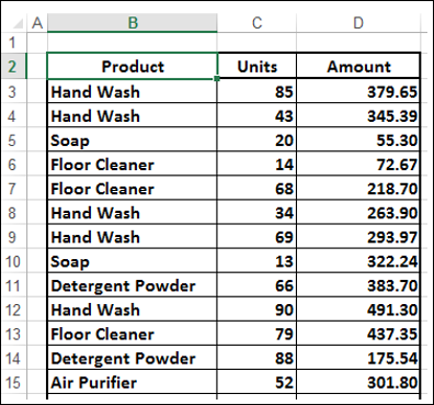
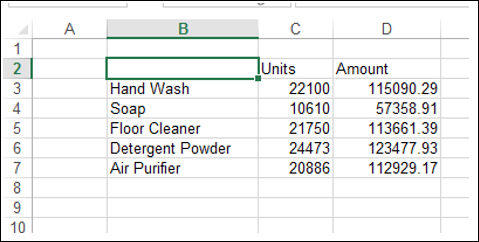
Suppose you have the sales data of various commodities from each of the regions – East, North, South, and West. You might need to consolidate this data and present a product wise summary of sales from time to time. Preparation includes the following −
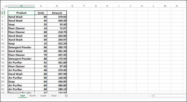
One worksheet per region – i.e. four worksheets with names East, North, South, and West. These could be in the same workbook or different workbooks.
Each worksheet has same layout, representing the details of product, number of units, and amount.
You need to consolidate the data product wise. Hence, ensure that the column with the label Product is the first column and it contains the Product labels.
Consolidating Data in the Same Workbook
If you have all the data, that you have to consolidate, in the same workbook, proceed as follows −
Step 1 − Ensure that data of each region is on a separate worksheet.
Step 2 − Add a new worksheet and name it Summary.
Step 3 − Click the Summary worksheet.
Step 4 − Click the cell where you want to place the summary results.
Step 5 − Click the DATA tab on the Ribbon.
Step 6 − Click the Consolidate button in the Data Tools group.
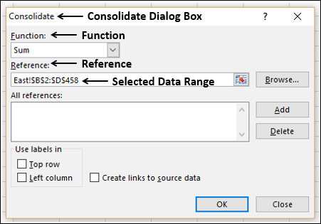
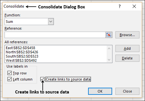
The Consolidate dialog box appears.
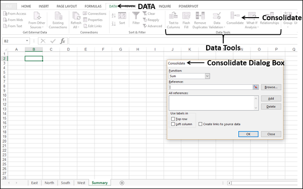
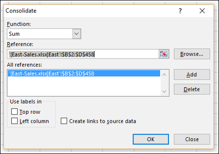
Step 7 − Select Sum from the dropdown list under Function.
Step 8 − Select the data from each worksheet as follows.
- Click the icon in the box under Reference.
- Select the worksheet – East.
- Select the data range.
- Again, click the icon in the box under Reference.
The selected range appears in the Reference box −
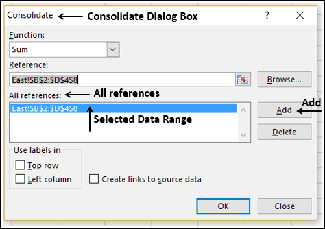
Step 9 − Click the Add button to the right of the box. The selected data range appears in the box under All References.
Step 10 − Repeat Steps 1-5 for the rest of the data worksheets – North, South, and West. The Consolidate dialog box looks as follows.
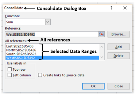
You can see that the data ranges appear worksheet wise in alphabetical order, in the box under All references.
Step 11 − Check the boxes Top row and Left column under Use labels in. Click OK.
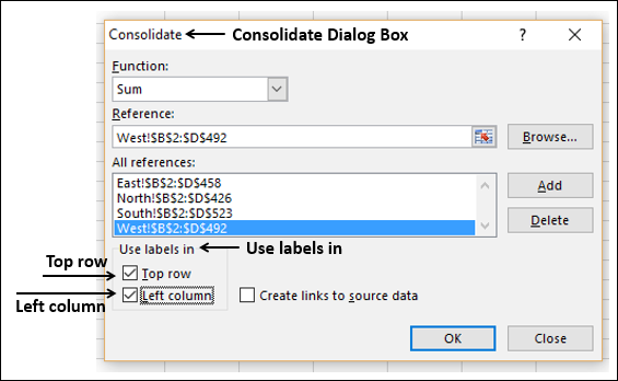
Your data is summarized product wise for the regions – East, North, South and West.
You can repeat the steps given above to refresh your summary results manually, whenever you need them.
Consolidating Data Automatically
Suppose you want your summary sheet to be updated automatically, whenever there are changes in the data. To accomplish this, you need to have links to the source data.
Step 1 − Check the box - Create links to source data in the Consolidate dialog box and click OK.
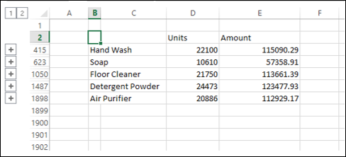
Your summary results appear with an outline as follows −
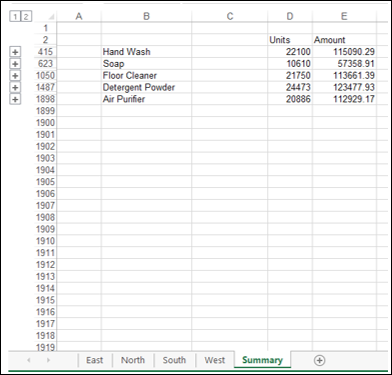
You will observe that a new column is inserted to the right of the column named Product.
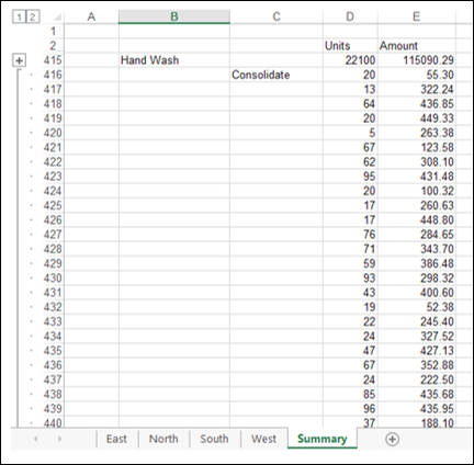
Step 2 − Click the + sign on the outline in the row containing the Product value named Soap. You can see that the new column contains the consolidated value for each set of product values, region wise.
Consolidating Data from Different Workbooks
In the previous example, all the data that you need to summarize is in the same workbook. However, it is likely that the data is maintained separately for each region and is updated region wise. In such a case, you can consolidate the data as follows −
Step 1 − Open the workbooks containing the data, say, workbooks – East-Sales, North-Sales, South-Sales and West-Sales.
Step 2 − Open a new workbook.
Step 3 − On a new worksheet, click a cell where you want the summary to appear.
Step 4 − Click the DATA tab on the Ribbon.
Step 5 − Click Consolidate in the Data Tools box.
A Consolidate dialog box appears. In the Consolidate dialog box −
- Select Sum from the dropdown list in the box under Function.
- Click the icon in the box under Reference.
- Select the workbook – East-Sales.xlsx.
- Select the data range.
- Again, click the icon in the box under Reference.
- Click the Add button to the right.
The Consolidate dialog box looks as follows −
- Click the icon to the right of the box under References.
- Select the workbook – North-Sales.xlsx.
- Select the data range.
- Again, click the icon to the right of the box under References.
- Click Add.
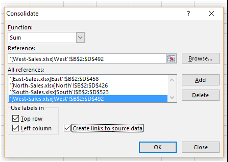
Step 6 − Repeat the steps 1–6 to add the data ranges from the workbooks – South-Sales.xlsx and West-Sales.xlsx.
Step 7 − Under Use labels in, check the following boxes.
- Top row.
- Left column.
Step 8 − Check the box Create links to source data.
Your Consolidate dialog box looks as follows −
Your data is summarized in your workbook.