- Excel Data Analysis Tutorial
- Excel Data Analysis - Home
- Data Analysis - Overview
- Data Analysis - Process
- Excel Data Analysis - Overview
- Working with Range Names
- Tables
- Cleaning Data with Text Functions
- Cleaning Data Contains Date Values
- Working with Time Values
- Conditional Formatting
- Sorting
- Filtering
- Subtotals with Ranges
- Quick Analysis
- Lookup Functions
- PivotTables
- Data Visualization
- Data Validation
- Financial Analysis
- Working with Multiple Sheets
- Formula Auditing
- Inquire
- Advanced Data Analysis
- Advanced Data Analysis - Overview
- Data Consolidation
- What-If Analysis
- What-If Analysis with Data Tables
- What-If Analysis Scenario Manager
- What-If Analysis with Goal Seek
- Optimization with Excel Solver
- Importing Data into Excel
- Data Model
- Exploring Data with PivotTables
- Exploring Data with Powerpivot
- Exploring Data with Power View
- Exploring Data Power View Charts
- Exploring Data Power View Maps
- Exploring Data PowerView Multiples
- Exploring Data Power View Tiles
- Exploring Data with Hierarchies
- Aesthetic Power View Reports
- Key Performance Indicators
- Excel Data Analysis Resources
- Excel Data Analysis - Quick Guide
- Excel Data Analysis - Resources
- Excel Data Analysis - Discussion
Excel Data Analysis - Formula Auditing
You might want to check formulas for accuracy or find the source of an error. Excel Formula Auditing commands provide you an easy way to find
- Which cells are contributing in the calculation of a formula in the active cell.
- Which formulas are referring to the active cell.
These findings are shown graphically by arrow lines that makes the visualization easy. You can display all the formulas in the active worksheet with a single command. If your formulas refer to cells in a different workbook, open that workbook also. Excel cannot go to a cell in a workbook that is not open.
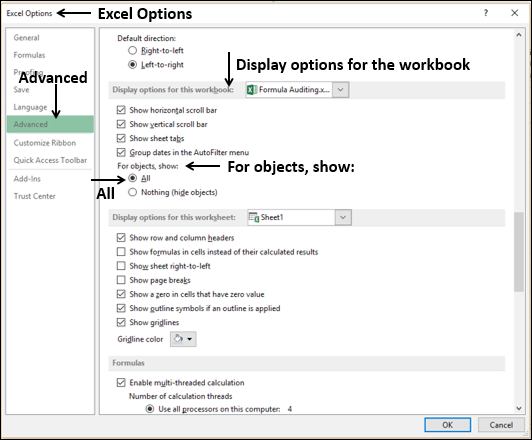
Setting the Display Options
You need to check whether the display options for the workbooks you are using are correctly set.
- Click FILE > Options.
- In the Excel Options dialog box, click Advanced.
- In Display options for the workbook −
- Select the workbook.
- Check that under For objects, show, All is selected.
- Repeat this step for all the workbooks you are auditing.
Tracing Precedents
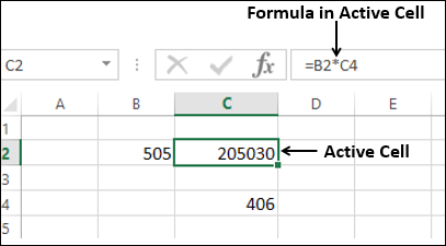
Precedent cells are those cells that are referred to by a formula in the active cell.
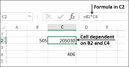
In the following example, the active cell is C2. In C2, you have the formula =B2*C4.
B2 and C4 are precedent cells for C2.
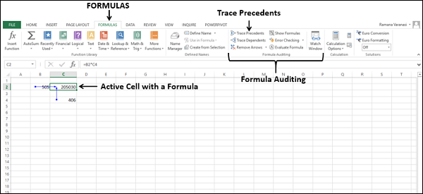
To trace the precedents of the cell C2,
- Click in the cell C2.
- Click the Formulas tab.
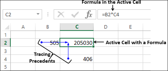
- Click Trace Precedents in the Formula Auditing group.
Two arrows, one from B2 to C2 and another from C4 to C2 will be displayed, tracing the precedents.
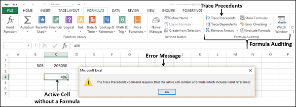
Note that for tracing precedents of a cell, the cell should have a formula with valid references. Otherwise, you will get an error message.
- Click in a cell that does not contain a formula or click in an empty cell.
- Click Trace Precedents in the Formula Auditing group.
You will get a message.
Removing Arrows
Click Remove Arrows in the Formula Auditing group.
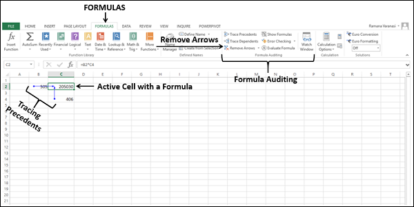
All the arrows in the worksheet will disappear.
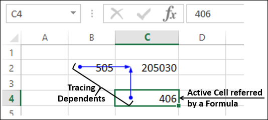
Tracing Dependents
Dependent cells contain formulas that refer to other cells. That means, if the active cell contributes to a formula in another cell, the other cell is a dependent cell on the active cell.
In the example below, C2 has the formula =B2*C4. Therefore, C2 is a dependent cell on the cells B2 and C4
To trace the dependents of the cell B2,
- Click in the cell B2.
- Click the Formulas tab.
- Click Trace Dependents in the Formula Auditing group.
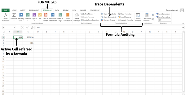
An arrow appears from B2 to C2, showing C2 is dependent on B2.
To trace the dependents of the cell C4 −
- Click in the cell C4.
- Click the Formula tab > Trace Dependents in the Formula Auditing group.
Another arrow appears from C4 to C2, showing C2 is dependent on C4 also.
Click Remove Arrows in the Formula Auditing group. All the arrows in the worksheet will disappear.
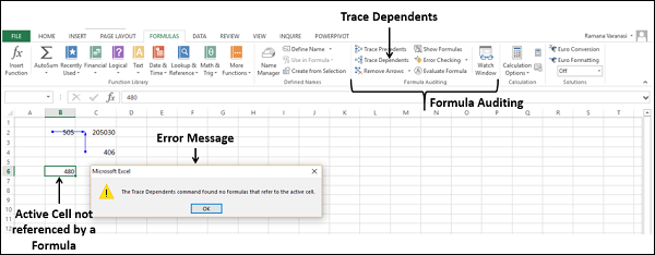
Note − For tracing dependents of a cell, the cell should be referenced by a formula in another cell. Otherwise, you will get an error message.
- Click in the cell B6 is not referenced by any formula or click in any empty cell.
- Click Trace Dependents in the Formula Auditing group. You will get a message.
Working with Formulae
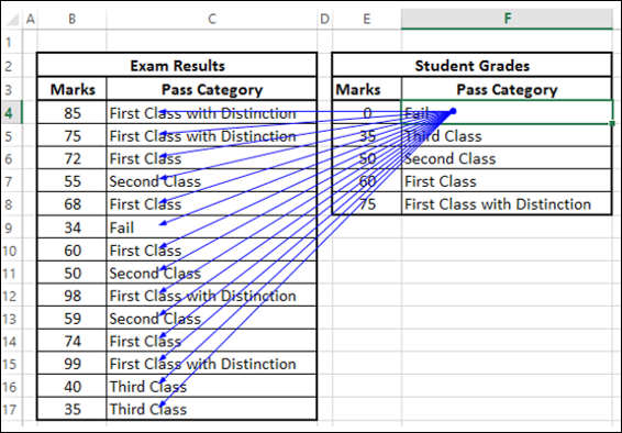
You have understood the concept of Precedents and Dependents. Now, consider a worksheet with several formulae.
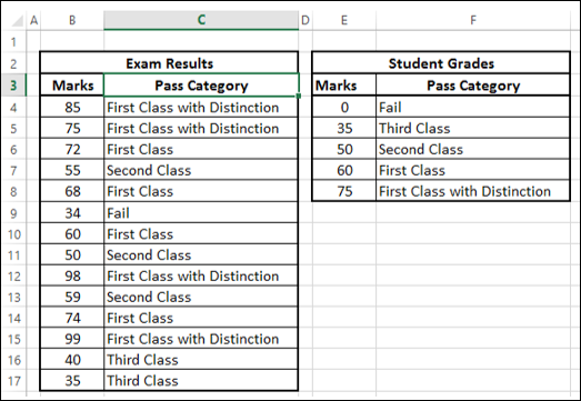
- Click in a cell under Pass Category in Exam Results table.
- Click Trace Precedents. The cell to its left (Marks) and the range E4:F8 will be mapped as the precedents.
- Repeat for all the cells under Pass Category in Exam Results table.
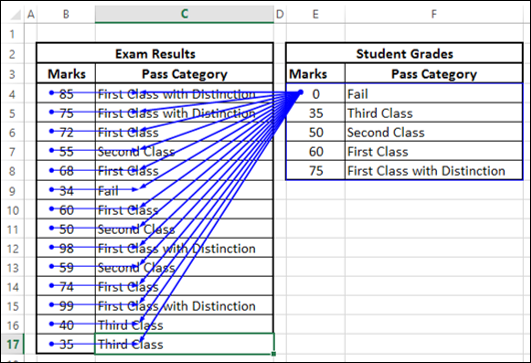
Click in a cell under Pass Category in Student Grades table.
Click Trace Dependents. All the cells under Pass Category in Exam Results table will be mapped as the dependents.
Showing Formulas
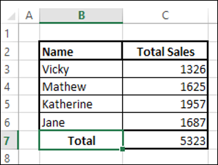
The worksheet below contains the summary of sales by the salespersons in the regions East, North, South, and West.
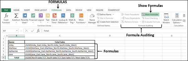
Click the FORMULAS tab on the Ribbon.
Click Show Formulas in the Formula Auditing group. The Formulas in the worksheet will appear, so that you will know which cells contain formulas and what the formulas are.
Click in a cell under TotalSales.
Click Trace Precedents. A worksheet icon appears at the end of the arrow. The worksheet icon indicates that the precedents are in a different worksheet.
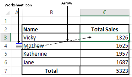
Double-click on the arrow. A Go TO dialog box appears, showing the precedents.
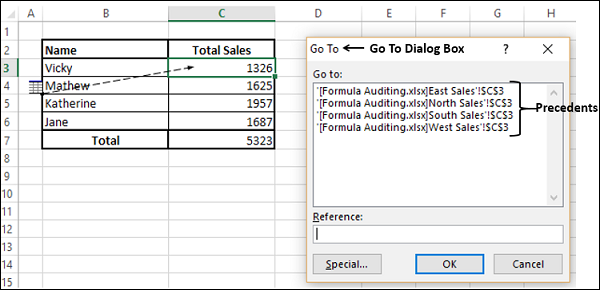
As you observe, there are four precedents, on four different worksheets.
- Click a reference of one of the precedents.
- The reference appears in the Reference box.
- Click OK. The worksheet containing that precedent appears.
Evaluating a Formula
To find how a complex formula in a cell works step by step, you can use Evaluate Formula command.
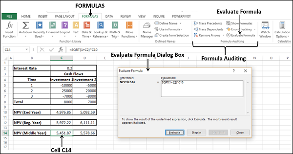
Consider the formula NPV (Middle Year) in the cell C14. The formula is
=SQRT (1 + C2)*C10
- Click in the cell C14.
- Click the FORMULAS tab on the Ribbon.
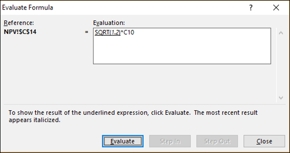
- Click Evaluate Formula in the Formula Auditing group. The Evaluate Formula dialog box appears.
In the Evaluate Formula dialog box, the formula is displayed in the box under Evaluation. By clicking the Evaluate button several times, the formula gets evaluated step-wise. The expression with an underline will always be executed next.
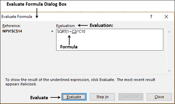
Here, C2 is underlined in the formula. So, it is evaluated in the next step. Click Evaluate.
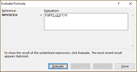
Cell C2 has value 0.2. Hence, C2 will be evaluated as 0.2. 1+0.2 is underlined showing it as the next step. Click Evaluate.
1+0.2 will be evaluated as 1.2. SQRT(1.2) is underlined showing it as next step. Click Evaluate.
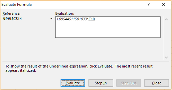
SQRT(1.2) will be evaluated as 1.09544511501033. C10 is underlined showing it as next step. Click Evaluate.
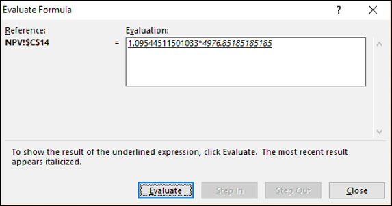
C10 will be evaluated as 4976.8518518515.
1.09544511501033*4976.8518518515 is underlined showing it as next step. Click Evaluate.
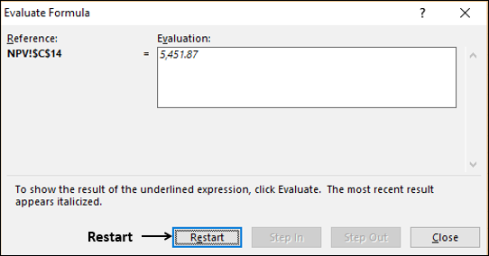
1.09544511501033*4976.8518518515 will be evaluated as 5,451.87.
There are no more expressions to evaluate and this is the answer. The Evaluate button will be changed to Restart button, indicating completion of evaluation.
Error Checking
It is a good practice to do an error check once your worksheet and/or workbook is ready with calculations.
Consider the following simple calculations.
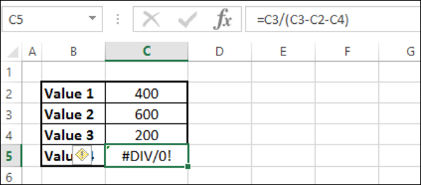
The calculation in the cell has resulted in the error #DIV/0!.
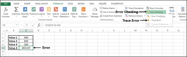
Click in the cell C5.
Click the FORMULAS tab on the Ribbon.
Click the arrow next to Error Checking in the Formula Auditing group. In the drop-down list, you will find that Circular References is deactivated, indicating that your worksheet has no circular references.
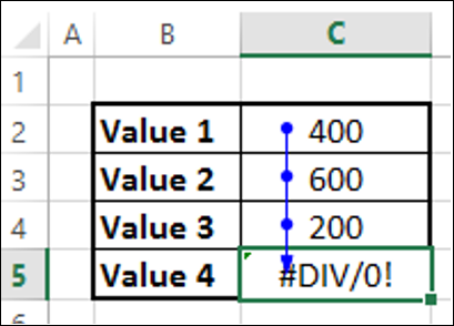
Select Trace Error from the drop-down list.
The cells needed to compute the active cell are indicated by blue arrows.
- Click Remove Arrows.
- Click the arrow next to Error Checking.
- Select Error Checking from the drop-down list.
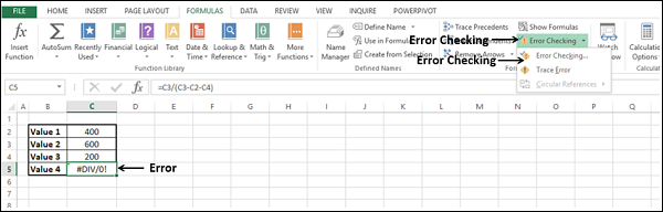
The Error Checking dialog box appears.
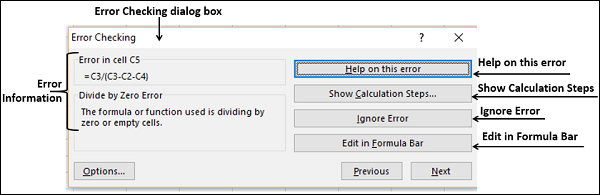
Observe the following −
If you click Help on this error, Excel help on the error will be displayed.
If you click Show Calculation Steps, Evaluate Formula dialog box appears.
If you click Ignore Error, the Error Checking dialog box closes and if you click Error Checking command again, it ignores this error.
If you click Edit in Formula Bar, you will be taken to the formula in the formula bar, so that you can edit the formula in the cell.