Excel Data Analysis - Data Validation

Data Validation is a very useful and easy to use tool in Excel with which you can set data validations on the data that is entered that is entered into your Worksheet.

For any cell on the worksheet, you can

Display an input message on what needs to be entered into it.
Restrict the values that get entered.
Provide a list of values to choose from.
Display an error message and reject an invalid data entry.

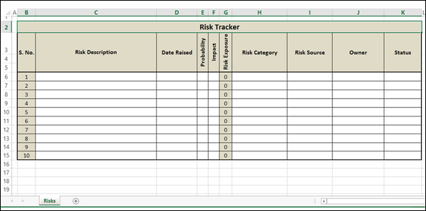
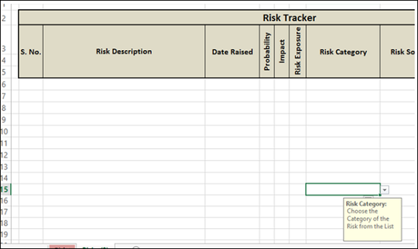
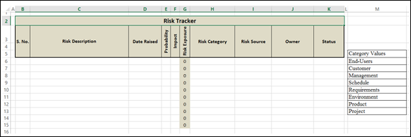
Consider the following Risk Tracker that can be used to enter and track the identified Risks information.

In this tracker, the data that is entered into the following columns is validated with preset data constraints and the entered data is accepted only when it meets the validation criteria. Otherwise, you will get an error message.

Probability
Impact
Risk Category
Risk Source
Status

The column Risk Exposure will have calculated values and you cannot enter any data. Even the column S. No. is set to have calculated values that are adjusted even if you delete a row.

Now, you will learn how to set up such a worksheet.

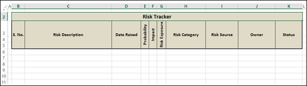
Prepare the Structure for the Worksheet

To prepare the structure for the worksheet −

Start with a blank worksheet.
Put the header in Row 2.
Put the column headers in Row 3.
For the column headers Probability, Impact and Risk Exposure −
- Right click on the cell.
- Click on Format Cells from drop down.
- In the Format Cells dialog box, click on Alignment tab.
- Type 90 under Orientation.
Merge and Centre the cells in Rows 3, 4, and 5 for each of the column headers.
Format Borders for the cells in Rows 2 – 5.
Adjust the row and column widths.

Your worksheet will look as follow −

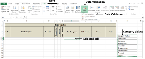
Set Valid Values for Risk Category

In the cells M5 – M13 enter the following values (M5 is heading and M6 - M13 are the values)

Category Values

End-Users

Customer

Management

Schedule

Environment

Product

Project

Click the first cell under the column Risk Category (H6).
Click DATA tab on the Ribbon.
Click Data Validation in the Data Tools group.
Select Data Validation… from the drop-down list.

The Data Validation dialog box appears.

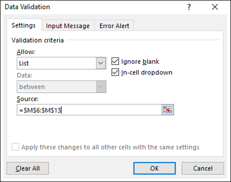
Click the Settings tab.
Under Validation criteria, in the Allow: drop-down list, Select the option List.

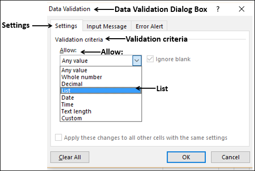
Select the range M6:M13 in the Source: box that appears.
Check the boxes Ignore blank and In-cell dropdown that appear.

Set Input Message for Risk Category

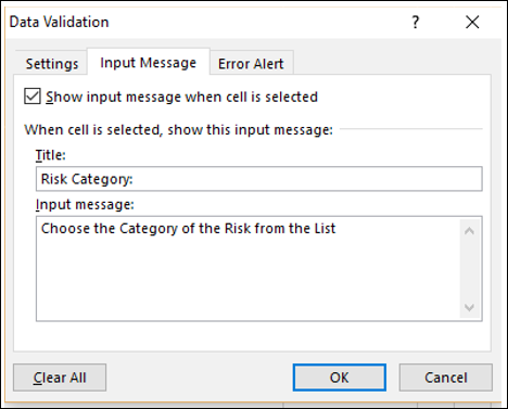
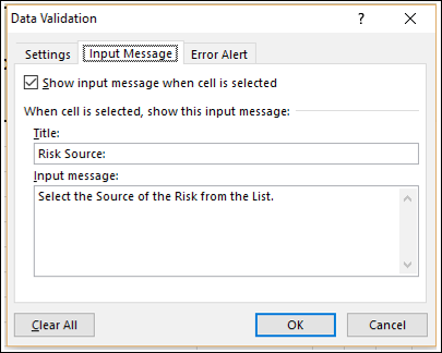
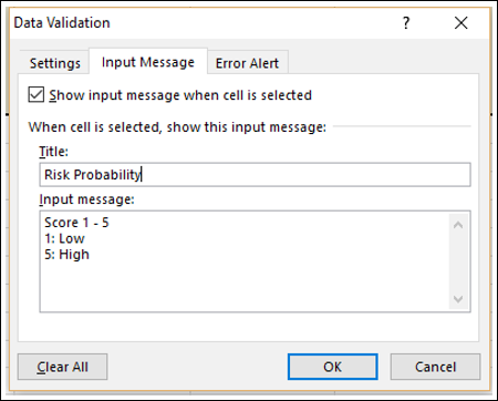
Click the Input Message tab in the Data Validation dialog box.
Check the box Show input message when cell is selected.
In the box under Title:, type Risk Category:
In the box under Input message: Choose the Category of the Risk from the List.

Set Error Alert for Risk Category

To set error alert −

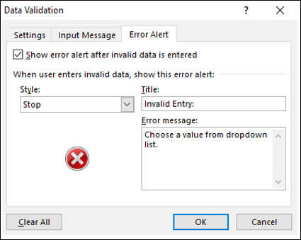
Click the Error Alert tab in the Data validation dialog box.
Check the box Show error alert after invalid data is entered.
Select Stop under Style: dropdown
In the box under Title:, type Invalid Entry:
In the box under Error message: type Choose a value from dropdown list.
Click OK.

Verify Data Validation for Risk Category

For the selected first cell under Risk Category,

Data Validation criteria is set
Input message is set
Error alert is set

Now, you can verify your settings.

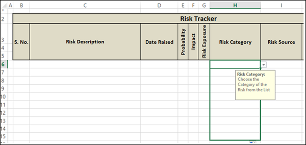
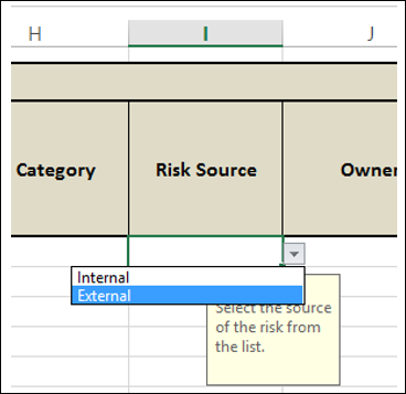
Click in the cell for which you have set Data Validation criteria. The Input message appears. The dropdown button appears on the right side of the cell.

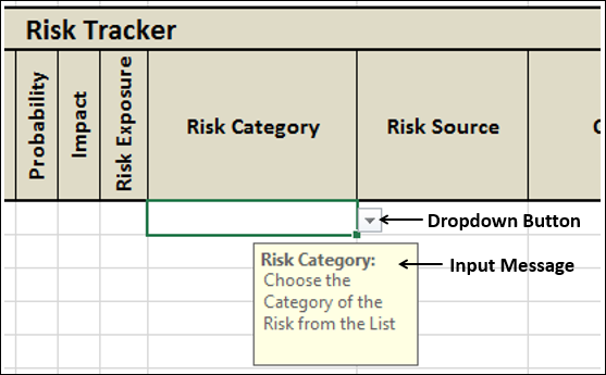
The input message is correctly displayed.

Click on the dropdown button on the right side of the cell. The drop-down list appears with the values that can be selected.
Cross-check the values in the drop-down list with those that are used to create the drop-down list.

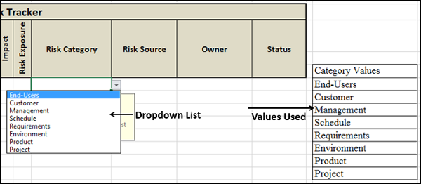
Both the sets of values match. Note that if the number of values is more, you will get a scroll-down bar on the right side of the dropdown list.

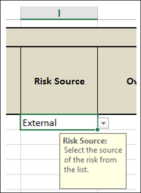
Select a value from the dropdown list. It appears in the cell.

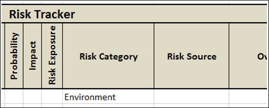
You can see that the selection of valid values is working fine.

Finally, try to enter an invalid entry and verify the Error alert.

Type People in the cell and press Enter. Error message that you have set for the cell will be displayed.

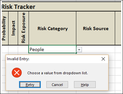
Verify the Error message.
You have an option to either Retry or Cancel. Verify both the options.

You have successfully set the Data Validation for the cell.

Note − It is very important to check the spelling and grammar of your messages.

Set Valid Criteria for the Risk Category Column

Now, you are ready to apply the Data Validation criteria to all the cells in the Risk Category column.

At this point, you need to remember two things −

You need to set the criteria for maximum number of cells that are possible to be used. In our example, it can vary from 10 – 100 based on where the worksheet will be used.
You should not set the criteria for unwanted range of cells or for the entire column. This will unnecessarily increases the file size. It is called excess formatting. If you get a worksheet from an outside source, you have to remove the excess formatting, which you will learn in the chapter on Inquire in this tutorial.

Follow the steps given below −

Set the validation criteria for 10 cells under Risk Category.
You can easily do this by clicking on the right-bottom corner of the first cell.
Hold on the + symbol that appears and pull it down.

Data Validation is set for all the selected cells.

Click the last column that is selected and verify.

Data Validation for the column Risk Category is complete.

Set Validation Values for Risk Source

In this case, we have only two values – Internal and External.

Click in the first cell under the column Risk Source (I6)
Click the DATA tab on the Ribbon
Click Data Validation in the Data Tools group
Select Data Validation… from the drop-down list.

Data Validation dialog box appears.

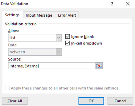
Click the Settings tab.
Under Validation criteria, in the Allow: drop-down list, select the option List.
Type Internal, External in the Source: box that appears.
Check the boxes Ignore blank and In-cell dropdown that appear.

Set Input Message for Risk Source.

Set Error Alert for Risk Source.

For the selected first cell under Risk Source −

Data Validation criteria is set
Input message is set
Error alert is set

Now, you can verify your settings.

Click in the cell for which you have set Data Validation criteria. Input message appears. The drop-down button appears on the right side of the cell.

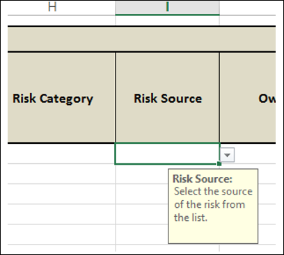
The input message is displayed correctly.

Click the drop-down arrow button on the right side of the cell. A drop-down list appears with the values that can be selected.
Check if the values are the same as you typed – Internal and External.

Both the sets of values match. Select a value from the drop-down list. It appears in the cell.

You can see that the selection of valid values is working fine. Finally, try to enter an invalid entry and verify the Error alert.

Type Financial in the cell and press Enter. Error message that you have set for the cell will be displayed.

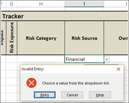
Verify the Error message. You have successfully set the Data Validation for the cell.
Set valid criteria for the Risk Source Column
Apply the Data Validation criteria to the cells I6 - I15 in the Risk Source column (i.e. same range as that of Risk Category column).

Data Validation is set for all the selected cells. Data Validation for the column Risk Source is complete.

Set Validation Values for Status

Repeat the same steps that you used for setting Validation values for Risk Source.
Set the List values as Open, Closed.
Apply the Data Validation criteria to the cells K6 - K15 in the Status column (i.e. same range as that of Risk Category column).

Data Validation is set for all the selected cells. Data Validation for the column status is complete.

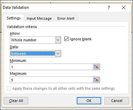
Set Validation Values for Probability

Risk Probability Score values are in the range 1-5, 1 being low and 5 being high. The value can be any integer between 1 and 5, both inclusive.

Click in the first cell under the column Risk Source (I6).
Click the DATA tab on the Ribbon.
Click Data Validation in the Data Tools group.
Select Data Validation… from the drop-down list.

The Data Validation dialog box appears.

Click the Settings tab.
Under Validation criteria, in the Allow: drop-down list, select Whole number.

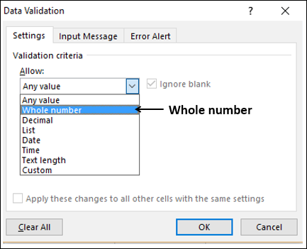
Select between under Data:
Type 1 in the box under Minimum:
Type 5 in the box under Maximum:

Set Input Message for Probability

Set Error Alert for Probability and click OK.

For the selected first cell under Probability,

Data Validation criteria is set.
Input message is set.
Error alert is set.

Now, you can verify your settings.

Click on the cell for which you have set Data Validation criteria. Input message appears. In this case, there will not be a dropdown button because the input values are set to be in a range and not from list.

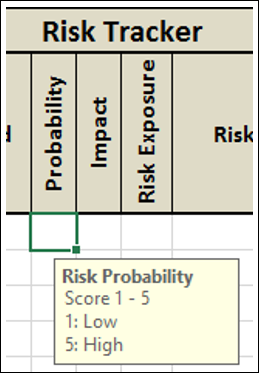
The input message is correctly displayed.

Enter an integer between 1 and 5 in the cell. It appears in the cell.

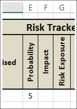
Selection of valid values is working fine. Finally, try to enter an invalid entry and verify the Error alert.

Type 6 in the cell and press Enter. The Error message that you have set for the cell will be displayed.

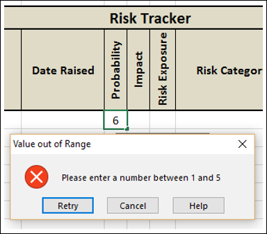
You have successfully set the Data Validation for the cell.

Set valid criteria for the Probability Column.
Apply the Data Validation criteria to the cells E6 - E15 in the Probability column (i.e. same range as that of Risk Category column).

Data Validation is set for all the selected cells. Data Validation for the column Probability is complete.

Set Validation Values for Impact

To set the validation values for Impact, repeat the same steps that you used for setting validation values for probability.

Apply the Data Validation criteria to the cells F6 - F15 in the Impact column (i.e. same range as that of Risk Category column).

Data Validation is set for all the selected cells. Data Validation for the column Impact is complete.

Set the Column Risk Exposure with Calculated Values

Risk Exposure is calculated as a product of Risk Probability and Risk Impact.

Risk Exposure = Probability * Impact

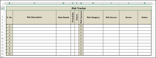
Type =E6*F6 in cell G6 and press Enter.

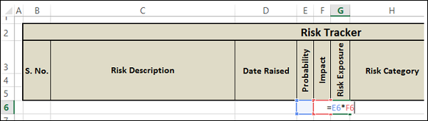
0 will be displayed in the cell G6 as E6 and F6 are empty.

Copy the formula in the cells G6 – G15. 0 will be displayed in the cells G6 - G15.

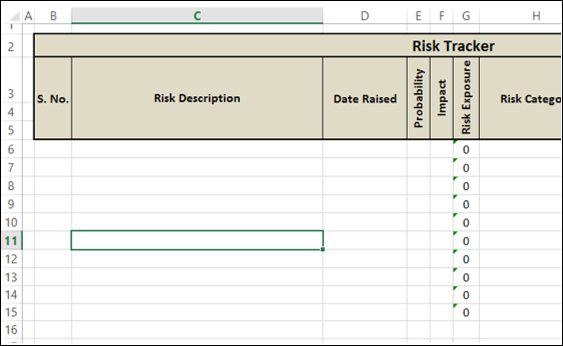
As the Risk Exposure column is meant for calculated values, you should not allow data entry in that column.

Select cells G6-G15
Right-click and in the dropdown list that appears, select Format Cells. The Format Cells dialog box appears.
Click the Protection tab.
Check the option Locked.

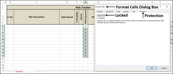
This is to ensure that data entry is not allowed in those cells. However, this will come into effect only when the worksheet is protected, which you will do as the last step after the worksheet is ready.

Click OK.
Shade the cells G6-G15 to indicate they are calculated values.

Format Serial Number Values

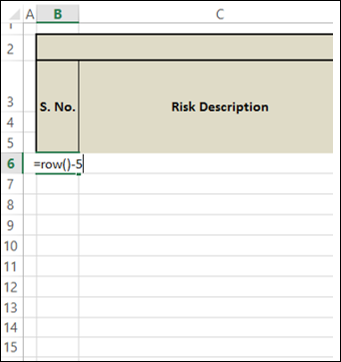
You can leave it to the user to fill in the S. No. Column. However, if you format the S. No. values, the worksheet looks more presentable. In addition, it shows for how many rows the worksheet is formatted.

Type =row()-5 in the cell B6 and press Enter.

1 will appear in cell B6. Copy the formula in the cells B6-B15. Values 1-10 appear.

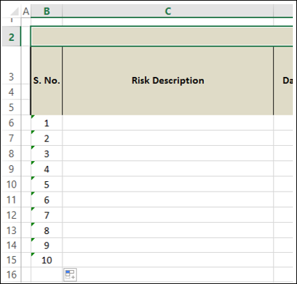
Shade the cells B6-B15.

Wrap-up

You are almost done with your project.

Hide Column M that contains Data Category values.
Format Borders for the cells B6-K16.

Right-click on the worksheet tab.
Select Protect Sheet from the menu.

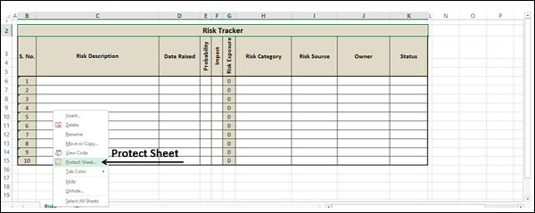
The Protect Sheet dialog box appears.

Check the option Protect worksheet and contents of locked cells.
Type in a password under Password to unprotect sheet −
- Password is case sensitive
- Protected sheet cannot be recovered if password is forgotten
- It is a good practice to keep a list of worksheet names and passwords somewhere
Under Allow all users of this worksheet to: check the box Select unlocked cells.

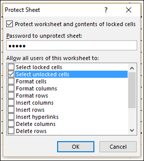
You have protected the locked cells in the column Risk Exposure from data entry and kept the rest of the unlocked cells editable. Click OK.

The Confirm Password dialog box appears.

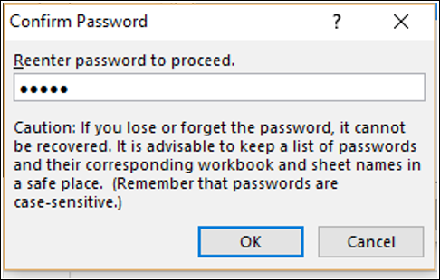
Re-enter the password.
Click OK.

Your worksheet with Data Validation set for selected cells is ready to use.