- Excel Data Analysis Tutorial
- Excel Data Analysis - Home
- Data Analysis - Overview
- Data Analysis - Process
- Excel Data Analysis - Overview
- Working with Range Names
- Tables
- Cleaning Data with Text Functions
- Cleaning Data Contains Date Values
- Working with Time Values
- Conditional Formatting
- Sorting
- Filtering
- Subtotals with Ranges
- Quick Analysis
- Lookup Functions
- PivotTables
- Data Visualization
- Data Validation
- Financial Analysis
- Working with Multiple Sheets
- Formula Auditing
- Inquire
- Advanced Data Analysis
- Advanced Data Analysis - Overview
- Data Consolidation
- What-If Analysis
- What-If Analysis with Data Tables
- What-If Analysis Scenario Manager
- What-If Analysis with Goal Seek
- Optimization with Excel Solver
- Importing Data into Excel
- Data Model
- Exploring Data with PivotTables
- Exploring Data with Powerpivot
- Exploring Data with Power View
- Exploring Data Power View Charts
- Exploring Data Power View Maps
- Exploring Data PowerView Multiples
- Exploring Data Power View Tiles
- Exploring Data with Hierarchies
- Aesthetic Power View Reports
- Key Performance Indicators
- Excel Data Analysis Resources
- Excel Data Analysis - Quick Guide
- Excel Data Analysis - Resources
- Excel Data Analysis - Discussion
Excel Data Analysis - Conditional Formatting
In Microsoft Excel, you can use Conditional Formatting for data visualization. You have to specify formatting for a cell range based on the contents of the cell range. The cells that meet the specified conditions would be formatted as you have defined.
Example
In a range containing the sales figures of the past quarter for a set of salespersons, you can highlight those cells representing who have met the defined target, say, $2500.
You can set the condition as total sales of the person >= $2500 and specify a color code green. Excel checks each cell in the range to determine whether the condition you specified, i.e., total sales of the person >= $2500 is satisfied.
Excel applies the format you chose, i.e. the green color to all the cells that satisfy the condition. If the content of a cell does not satisfy the condition, the formatting of the cell remains unchanged. The result is as expected, only for the salespersons who have met the target, the cells are highlighted in green – a quick visualization of the analysis results.
You can specify any number of conditions for formatting by specifying Rules. You can pick up the rules that match your conditions from
- Highlight cells rules
- Top / Bottom rules
You can also define your own rules. You can −
- Add a rule
- Clear an existing rule
- Manage the defined rules
Further, you have several formatting options in Excel to choose the ones that are appropriate for your Data Visualization −
- Data Bars
- Color Scales
- Icon Sets
Conditional formatting has been promoted over the versions Excel 2007, Excel 2010, Excel 2013. The examples you find in this chapter are from Excel 2013.
In the following sections, you will understand the conditional formatting rules, formatting options and how to work with rules.
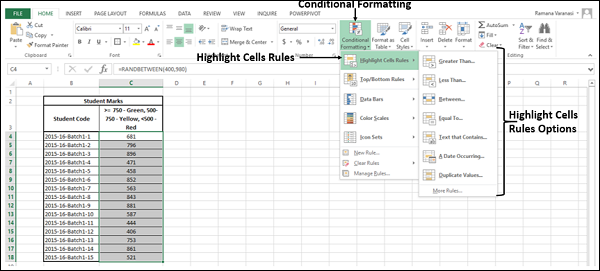
Highlight Cells Rules
You can use Highlight Cells rule to assign a format to cells whose contents meet any of the following criteria −
- Numbers within a given numerical range −
- Greater Than
- Less Than
- Between
- Equal To
- Text that contains a given text string.
- Date occurring within a given range of dates relative to the current date −
- Yesterday
- Today
- Tomorrow
- In the last 7 days
- Last week
- This week
- Next week
- Last month
- This Month
- Next month
- Values that are duplicate or unique.
Follow the steps to conditionally format cells −
Select the range to be conditionally formatted.
Click Conditional Formatting in the Styles group under Home tab.
Click Highlight Cells Rules from the drop-down menu.
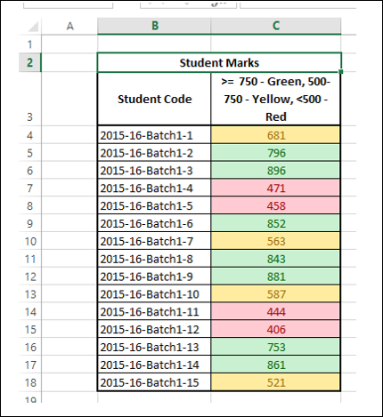
Click Greater Than and specify >750. Choose green color.
Click Less Than and specify < 500. Choose red color.
Click Between and specify 500 and 750. Choose yellow color.
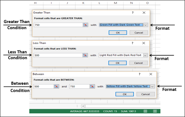
The data will be highlighted based on the given conditions and the corresponding formatting.
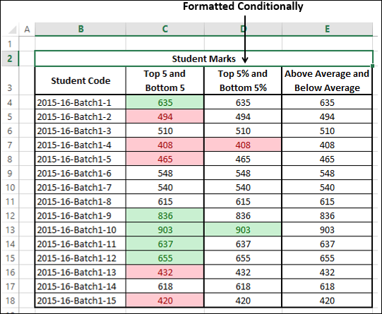
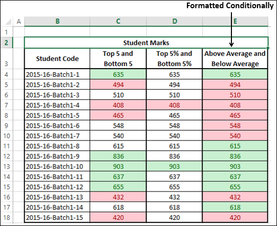
Top / Bottom Rules
You can use Top / Bottom Rules to assign a format to cells whose contents meet any of the following criteria −
Top 10 items − Cells that rank in the top N, where 1 <= N <= 1000.
Top 10% − Cells that rank in the top n%, where 1 <= n <= 100.
Bottom 10 items − Cells that rank in the bottom N, where 1 <= N <= 1000.
Bottom 10% − Cells that rank in the bottom n%, where 1 <= n <= 100.
Above average − Cells that are above average for the selected range.
Below average − Cells that are below average for the selected range.
Follow the steps given below to assign the Top/Bottom rules.
Select the range to be conditionally formatted.
Click Conditional Formatting in the Styles group under Home tab.
Click Top/Bottom Rules from the drop-down menu. Top/Bottom rules options appear.
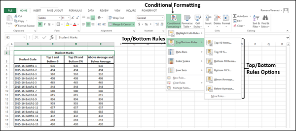
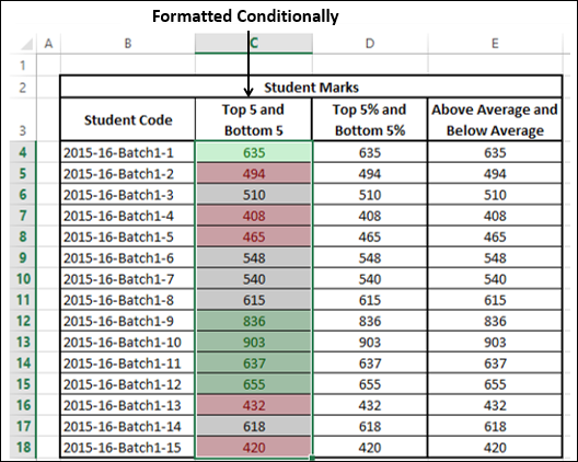
Click Top Ten Items and specify 5. Choose green color.
Click Bottom Ten Items and specify 5. Choose red color.
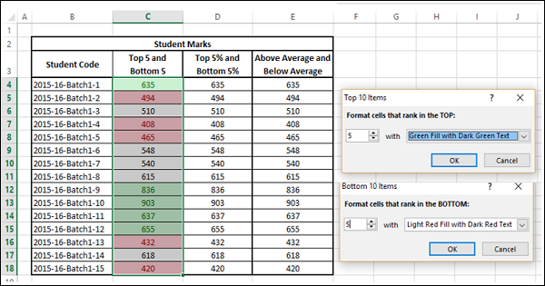
The data will be highlighted based on the given conditions and the corresponding formatting.
Repeat the first three steps given above.
Click Top Ten% and specify 5. Choose green color.
Click Bottom Ten% and specify 5. Choose red color.
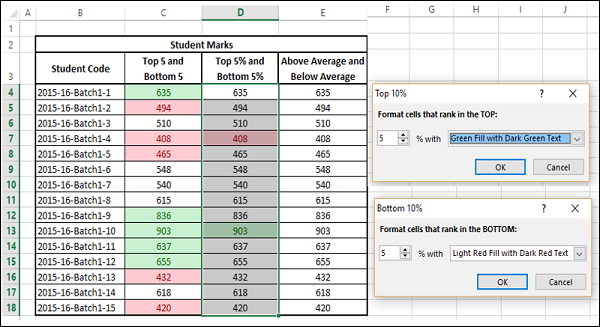
The data will be highlighted based on the given conditions and the corresponding formatting.
Repeat the first three steps given above.
Click Above Average. Choose green color.
Click Below Average. Choose red color.
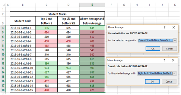
The data will be highlighted based on the given conditions and the corresponding formatting.
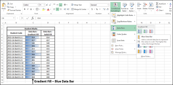
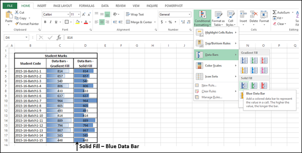
Data Bars
You can use colored Data Bars to see the value in a cell relative to the values in the other cells. The length of the data bar represents the value in the cell. A longer bar represents a higher value, and a shorter bar represents a lower value. You have six solid colors to choose from for the data bars – blue, green, red, yellow, light blue and purple.
Data bars are helpful in visualizing the higher, lower and intermediate values when you have large amounts of data. Example - Day temperatures across regions in a particular month. You can use gradient fill color bars to visualize the value in a cell relative to the values in other cells. You have six Gradient Colors to choose from for the Data Bars – Blue, Green, Red, Yellow, Light Blue and Purple.
Select the range to be formatted conditionally.
Click Conditional Formatting in the Styles group under Home tab.
Click Data Bars from the drop-down menu. The Gradient Fill options and Fill options appear.
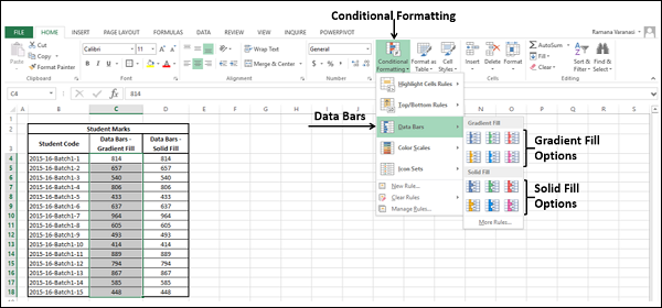
Click the blue data bar in the Gradient Fill options.
Repeat the first three steps.
Click the blue data bar in the Solid Fill options.
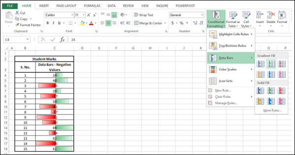
You can also format data bars such that the data bar starts in the middle of the cell, and stretches to the left for negative values and stretches to the right for positive values.
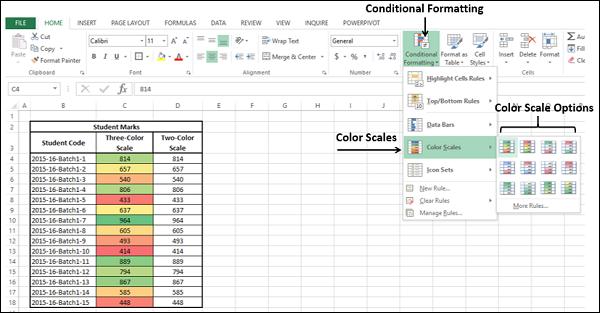
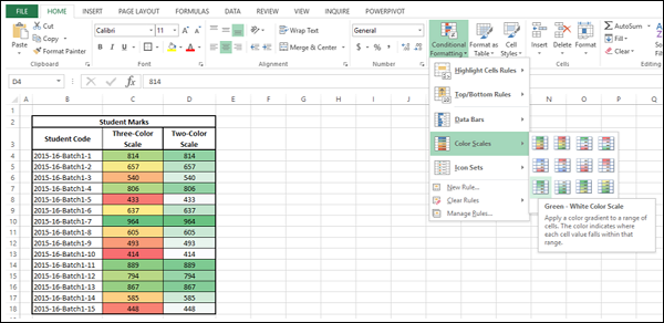
Color Scales
You can use Color Scales to see the value in a cell relative to the values in the other cells in a given range. As in the case of Highlight Cells Rules, a Color Scale uses cell shading to display the differences in cell values. A color gradient will be applied to a range of cells. The color indicates where each cell value falls within that range.
You can choose from −
- Three - Color Scale −
- Green – Yellow – Red Color Scale
- Red – Yellow – Green Color Scale
- Green – White – Red Color Scale
- Red – White – Green Color Scale
- Blue – White – Red Color Scale
- Red – White – Blue Color Scale
- Two-Color Scale −
- White – Red Color Scale
- Red – White Color Scale
- Green – White Color Scale
- White – Green Color Scale
- Green – Yellow Color Scale
- Yellow – Green Color Scale
Follow the steps given below −
Select the Range to be conditionally formatted.
Click Conditional Formatting in the Styles group under Home tab.
Click Color Scales from the drop-down menu. The Color Scale options appear.
Click the Green – Yellow – Red Color Scale.
The Data will be highlighted based on the Green – Yellow – Red color scale in the selected range.
- Repeat the first three steps.
- Click the Green – White color scale.
The data will be highlighted based on the Green – White color scale in the selected range.
Icon Sets
You can use the icon sets to visualize numerical differences. The following icon sets are available −
As you observe, an icon set consists of three to five symbols. You can define criteria to associate an icon with each value in a cell range. For example, a red down arrow for small numbers, a green up arrow for large numbers, and a yellow horizontal arrow for intermediate values.
Select the range to be conditionally formatted.
Click Conditional Formatting in the Styles group under Home tab.
Click Icon Sets from the drop-down menu. The Icon Sets options appear.
Click the colored three arrows.
Colored Arrows appear next to the Data based on the Values in the selected range.
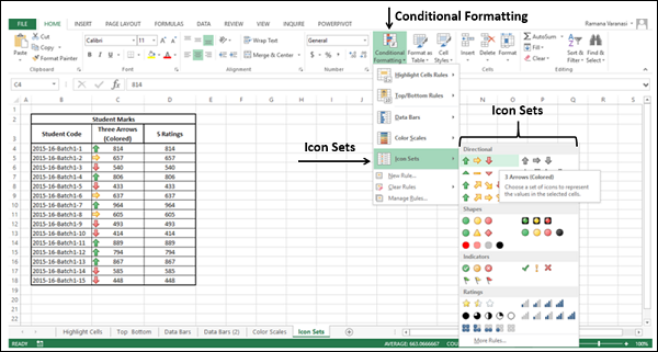
Repeat the first three steps. The Icon Sets options appear.
Select 5 Ratings. The Rating Icons appear next to the data based on the values in the selected range.
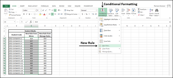
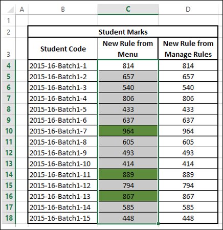
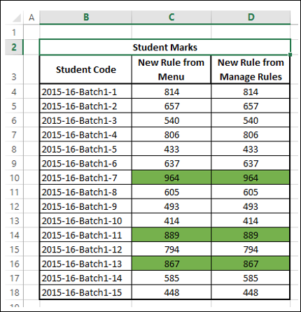
New Rule
You can use New Rule to create your own formula as a condition to format a cell as you define.
There are two ways to use New Rule −
With New Rule option from the drop-down menu
With New Rule button in Manage Rules dialog box
With New Rule option from the Drop-Down Menu
Select the Range to be conditionally formatted.
Click Conditional Formatting in the Styles group under Home tab.
Click New Rule from the drop-down menu.
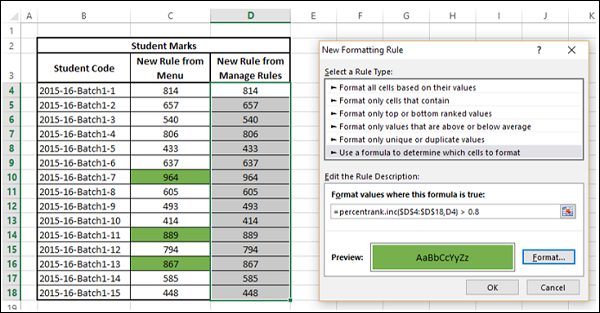
The New Formatting Rule dialog box appears.
From the Select a Rule Type Box, select Use a formula to determine which cells to format. Edit the Rule Description box appears.
In the format values where this formula is true: type the formula.
Click the format button and click OK.
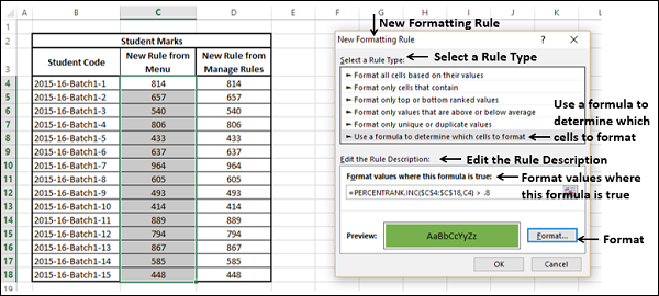
Cells that contain values with the formula TRUE, are formatted as defined.
With New Rule Button in Manage Rules dialog box
Select the range to be conditionally formatted.
Click Conditional Formatting in the Styles group under Home tab.
Click Manage Rules from the drop-down menu.
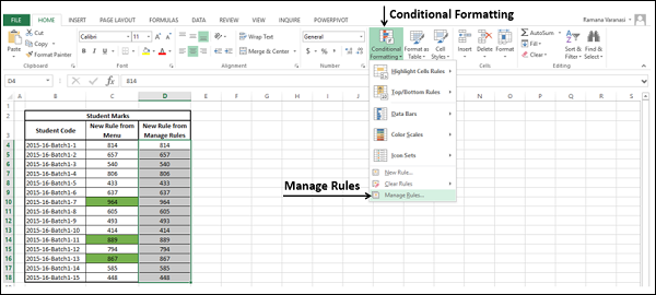
The Conditional Formatting Rules Manager dialog box appears.
Click the New Rule button.
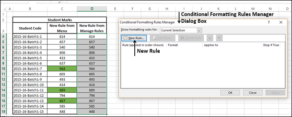
The New Formatting Rule dialog box appears.
Repeat the Steps given above to define your formula and format.
The Conditional Formatting Rules Manager dialog box appears with defined New Rule highlighted. Click the Apply button.
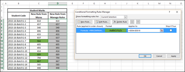
Cells that contain values with the formula TRUE, are formatted as defined.
Clear Rules
You can Clear Rules to delete all conditional formats you have created for
- Selected cells
- Current Worksheet
- Selected Table
- Selected PivotTable
Follow the given steps −
Select the Range / Click on a Worksheet / Click the table > PivotTable where conditional formatting rules need to be removed.
Click Conditional Formatting in the Styles group under Home tab.
Click Clear Rules from the drop-down menu. The Clear rules options appear.
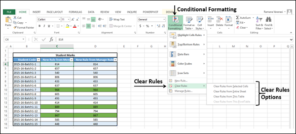
Select the appropriate option. The conditional formatting is cleared from the Range / Worksheet / Table / PivotTable.
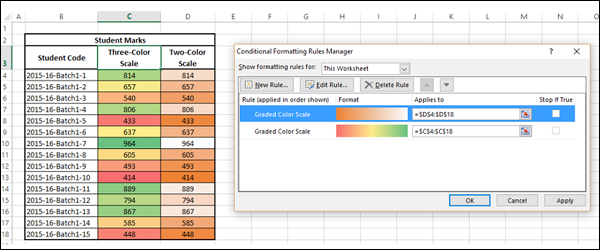
Manage Rules
You can Manage Rulesfrom the Conditional Formatting Rules Manager window. You can see formatting rules for the current selection, for the entire current worksheet, for the other worksheets in the workbook or the tables or PivotTables in the workbook.
Click Conditional Formatting in the Styles group under Home tab.
Click Manage Rules from the drop-down menu.
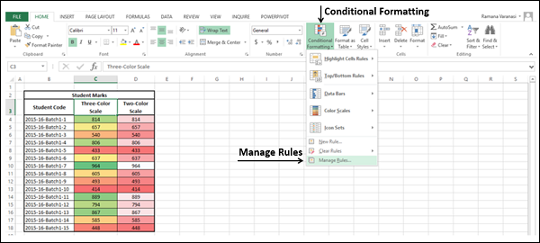
The Conditional Formatting Rules Manager dialog box appears.
Click the arrow in the List Box next to Show formatting rules for Current Selection, This Worksheet and other Sheets, Tables, PivotTable if exist with Conditional Formatting Rules, appear.
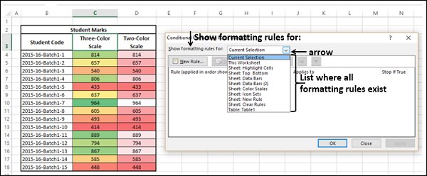
Select This Worksheet from the drop-down list. Formatting Rules on the current Worksheet appear in the order that they will be applied. You can change this order by using the up and down arrows.
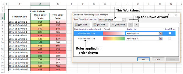
You can add a New Rule, Edit a Rule and Delete a Rule.
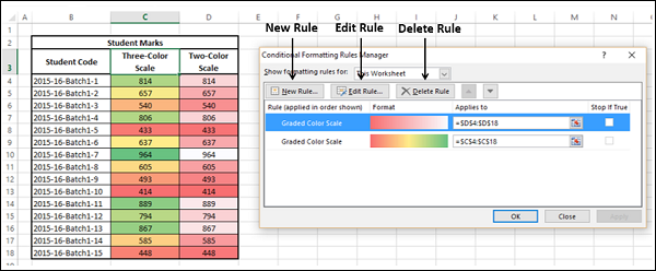
You have already seen New Rule in the earlier section. You can delete a rule by selecting the Rule and clicking Delete Rule. The highlighted Rule is deleted.
To edit a Rule, select the RULE and click on Edit Rule. Edit Formatting Rule dialog box appears.
You can
Select a Rule Type
Edit the Rule Description
Edit Formatting
Once you are done with the changes, click OK.
The changes for the Rule will be reflected in the Conditional Formatting Rules Manager dialog box. Click Apply.
The data will be highlighted based on the modified Conditional Formatting Rules.