- Analog Communication - Home
- Introduction
- Modulation
- Amplitude Modulation
- Numerical Problems 1
- AM Modulators
- AM Demodulators
- DSBSC Modulation
- DSBSC Modulators
- DSBSC Demodulators
- SSBSC Modulation
- SSBSC Modulators
- SSBSC Demodulator
- VSBSC Modulation
- Angle Modulation
- Numerical Problems 2
- FM Modulators
- FM Demodulators
- Multiplexing
- Noise
- SNR Calculations
- Transmitters
- Receivers
- Sampling
- Pulse Modulation
- Transducers
Analog Communication - Sampling
So far, we have discussed about continuous-wave modulation. We will discuss about pulse modulation in the next chapter. These pulse modulation techniques deal with discrete signals. So, now let us see how to convert a continuous time signal into a discrete one.
The process of converting continuous time signals into equivalent discrete time signals, can be termed as Sampling. A certain instant of data is continually sampled in the sampling process.
The following figure shows a continuous-time signal x(t) and the corresponding sampled signal xs(t). When x(t) is multiplied by a periodic impulse train, the sampled signal xs(t) is obtained.
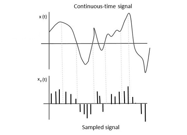
A sampling signal is a periodic train of pulses, having unit amplitude, sampled at equal intervals of time $T_s$, which is called as sampling time. This data is transmitted at the time instants $T_s$ and the carrier signal is transmitted at the remaining time.
Sampling Rate
To discretize the signals, the gap between the samples should be fixed. That gap can be termed as the sampling period $T_s$. Reciprocal of the sampling period is known as sampling frequency or sampling rate $f_s$.
Mathematically, we can write it as
$$f_s= \frac{1}{T_s}$$
Where,
$f_s$ is the sampling frequency or the sampling rate
$T_s$ is the sampling period
Sampling Theorem
The sampling rate should be such that the data in the message signal should neither be lost nor it should get over-lapped. The sampling theorem states that, a signal can be exactly reproduced if it is sampled at the rate $f_s$, which is greater than or equal to twice the maximum frequency of the given signal W.
Mathematically, we can write it as
$$f_s\geq 2W$$
Where,
$f_s$ is the sampling rate
$W$ is the highest frequency of the given signal
If the sampling rate is equal to twice the maximum frequency of the given signal W, then it is called as Nyquist rate.
The sampling theorem, which is also called as Nyquist theorem, delivers the theory of sufficient sample rate in terms of bandwidth for the class of functions that are bandlimited.
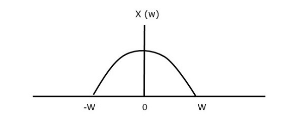
For continuous-time signal x(t), which is band-limited in the frequency domain is represented as shown in the following figure.
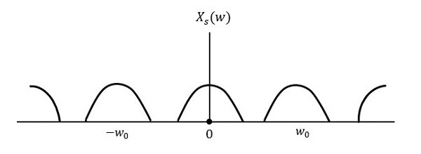
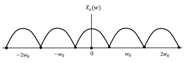
If the signal is sampled above Nyquist rate, then the original signal can be recovered. The following figure explains a signal, if sampled at a higher rate than 2w in the frequency domain.
If the same signal is sampled at a rate less than 2w, then the sampled signal would look like the following figure.
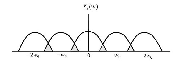
We can observe from the above pattern that there is over-lapping of information, which leads to mixing up and loss of information. This unwanted phenomenon of over-lapping is called as Aliasing.
Aliasing can be referred to as the phenomenon of a high-frequency component in the spectrum of a signal, taking on the identity of a low-frequency component in the spectrum of its sampled version.
Hence, the sampling rate of the signal is chosen to be as Nyquist rate. If the sampling rate is equal to twice the highest frequency of the given signal W, then the sampled signal would look like the following figure.
In this case, the signal can be recovered without any loss. Hence, this is a good sampling rate.
