- Excel Data Analysis - Home
- Data Analysis - Overview
- Data Analysis - Process
- Excel Data Analysis - Overview
- Working with Range Names
- Tables
- Cleaning Data with Text Functions
- Cleaning Data Contains Date Values
- Working with Time Values
- Conditional Formatting
- Sorting
- Filtering
- Subtotals with Ranges
- Quick Analysis
- Lookup Functions
- PivotTables
- Data Visualization
- Data Validation
- Financial Analysis
- Working with Multiple Sheets
- Formula Auditing
- Inquire
- Advanced Data Analysis - Overview
- Data Consolidation
- What-If Analysis
- What-If Analysis with Data Tables
- What-If Analysis Scenario Manager
- What-If Analysis with Goal Seek
- Optimization with Excel Solver
- Importing Data into Excel
- Data Model
- Exploring Data with PivotTables
- Exploring Data with Powerpivot
- Exploring Data with Power View
- Exploring Data Power View Charts
- Exploring Data Power View Maps
- Exploring Data PowerView Multiples
- Exploring Data Power View Tiles
- Exploring Data with Hierarchies
- Aesthetic Power View Reports
- Key Performance Indicators
- Excel Data Analysis Resources
- Excel Data Analysis - Quick Guide
- Excel Data Analysis - Resources
- Excel Data Analysis - Discussion
What-If Analysis with Data Tables
With a Data Table in Excel, you can easily vary one or two inputs and perform What-if analysis. A Data Table is a range of cells in which you can change values in some of the cells and come up with different answers to a problem.
There are two types of Data Tables −
- One-variable Data Tables
- Two-variable Data Tables
If you have more than two variables in your analysis problem, you need to use Scenario Manager Tool of Excel. For details, refer to the chapter What-If Analysis with Scenario Manager in this tutorial.
One-variable Data Tables
A one-variable Data Table can be used if you want to see how different values of one variable in one or more formulas will change the results of those formulas. In other words, with a one-variable Data Table, you can determine how changing one input changes any number of outputs. You will understand this with the help of an example.
Example
There is a loan of 5,000,000 for a tenure of 30 years. You want to know the monthly payments (EMI) for varied interest rates. You also might be interested in knowing the amount of interest and Principal that is paid in the second year.
Analysis with One-variable Data Table
Analysis with one-variable Data Table needs to be done in three steps −
Step 1 − Set the required background.
Step 2 − Create the Data Table.
Step 3 − Perform the Analysis.
Let us understand these steps in detail −
Step 1: Set the required background
Assume that the interest rate is 12%.
List all the required values.
Name the cells containing the values, so that the formulas will have names instead of cell references.
Set the calculations for EMI, Cumulative Interest and Cumulative Principal with the Excel functions PMT, CUMIPMT and CUMPRINC respectively.
Your worksheet should look as follows −
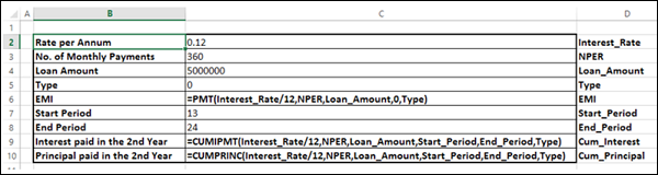
You can see that the cells in column C are named as given in the corresponding cells in column D.
Step 2: Create the Data Table
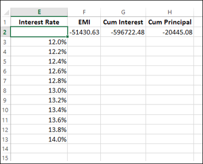
Type the list of values i.e. interest rates that you want to substitute in the input cell down the column E as follows −
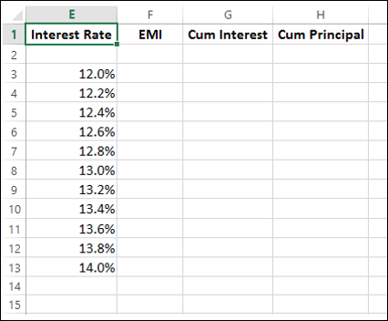
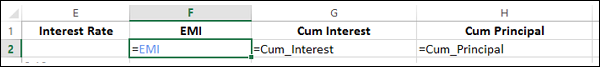
Type the first function (PMT) in the cell one row above and one cell to the right of the column of values. Type the other functions (CUMIPMT and CUMPRINC) in the cells to the right of the first function.
Now, the two rows above the Interest Rate values look as follows −
As you observe, there is an empty row above the Interest Rate values. This row is for the formulas that you want to use.
The Data Table looks as given below −
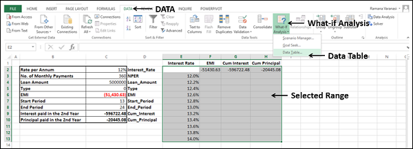
Step 3: Do the analysis with the What-If Analysis Data Table Tool
Select the range of cells that contains the formulas and values that you want to substitute, i.e. select the range E2:H13.
Click the DATA tab on the Ribbon.
Click What-if Analysis in the Data Tools group.
Select Data Table in the dropdown list.
Data Table dialog box appears.
- Click the icon in the Column input cell box.
- Click the cell Interest_Rate, which is C2.
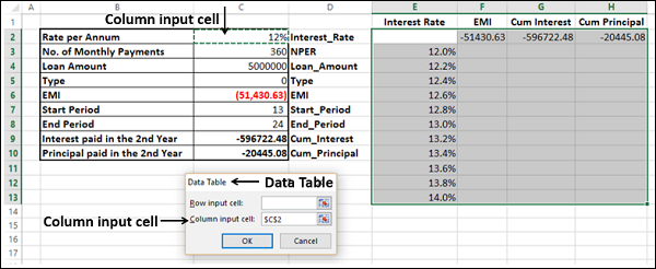
You can see that the Column input cell is taken as $C$2. Click OK.
The Data Table is filled with the calculated results for each of the input values as shown below −
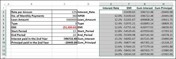
If you can pay an EMI of 54,000, you can observe that the interest rate of 12.6% is suitable for you.
Two-variable Data Tables
A two-variable Data Table can be used if you want to see how different values of two variables in a formula will change the results of that formula. In other words, with a twovariable Data Table, you can determine how changing two inputs changes a single output. You will understand this with the help of an example.
Example
There is a loan of 50,000,000. You want to know how different combinations of interest rates and loan tenures will affect the monthly payment (EMI).
Analysis with Two-variable Data Table
Analysis with two-variable Data Table needs to be done in three steps −
Step 1 − Set the required background.
Step 2 − Create the Data Table.
Step 3 − Perform the Analysis.
Step 1: Set the required background
Assume that the interest rate is 12%.
List all the required values.
Name the cells containing the values, so that the formula will have names instead of cell references.
Set the calculation for EMI with the Excel function PMT.
Your worksheet should look as follows −
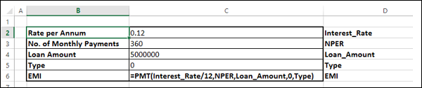
You can see that the cells in the column C are named as given in the corresponding cells in the column D.
Step 2: Create the Data Table
Type =EMI in cell F2.
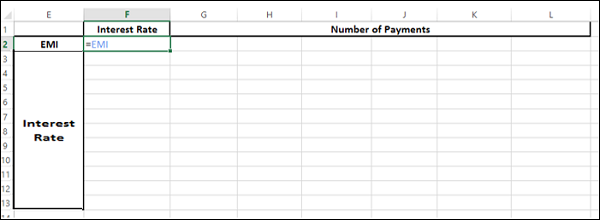
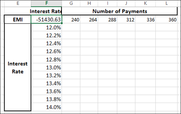
Type the first list of input values, i.e. interest rates down the column F, starting with the cell below the formula, i.e. F3.
Type the second list of input values, i.e. number of payments across row 2, starting with the cell to the right of the formula, i.e. G2.
The Data Table looks as follows −
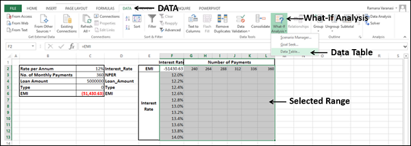
Do the analysis with the What-If Analysis Tool Data Table
Select the range of cells that contains the formula and the two sets of values that you want to substitute, i.e. select the range F2:L13.
Click the DATA tab on the Ribbon.
Click What-if Analysis in the Data Tools group.
Select Data Table from the dropdown list.
Data Table dialog box appears.
- Click the icon in the Row input cell box.
- Click the cell NPER, which is C3.
- Again, click the icon in the Row input cell box.
- Next, click the icon in the Column input cell box.
- Click the cell Interest_Rate, which is C2.
- Again, click the icon in the Column input cell box.
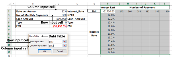
You will see that the Row input cell is taken as $C$3 and the Column input cell is taken as $C$2. Click OK.
The Data Table gets filled with the calculated results for each combination of the two input values −
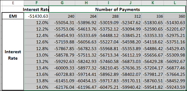
If you can pay an EMI of 54,000, the interest rate of 12.2% and 288 EMIs are suitable for you. This means the tenure of the loan would be 24 years.
Data Table Calculations
Data Tables are recalculated each time the worksheet containing them is recalculated, even if they have not changed. To speed up the calculations in a worksheet that contains a Data Table, you need to change the calculation options to Automatically Recalculate the worksheet but not the Data Tables, as given in the next section.
Speeding up the Calculations in a Worksheet
You can speed up the calculations in a worksheet containing Data Tables in two ways −
- From Excel Options.
- From the Ribbon.
From Excel Options
- Click the FILE tab on the Ribbon.
- Select Options from the list in the left pane.
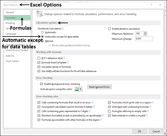
Excel Options dialog box appears.
From the left pane, select Formulas.
Select the option Automatic except for data tables under Workbook Calculation in the Calculation options section. Click OK.
From the Ribbon
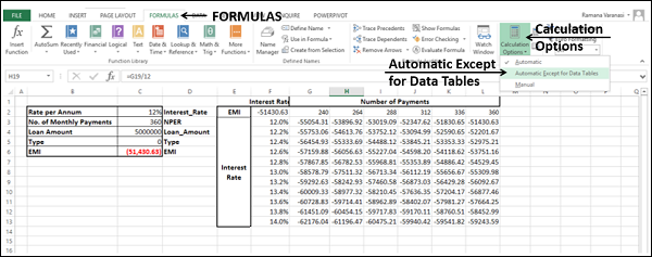
Click the FORMULAS tab on the Ribbon.
Click the Calculation Options in the Calculations group.
Select Automatic Except for Data Tables in the dropdown list.