Optimization with Excel Solver

Solver is a Microsoft Excel add-in program you can use for optimization in what-if analysis.

According to O'Brien and Marakas, optimization analysis is a more complex extension of goal-seeking analysis. Instead of setting a specific target value for a variable, the goal is to find the optimum value for one or more target variables, under certain constraints. Then, one or more other variables are changed repeatedly, subject to the specified constraints, until you discover the best values for the target variables.

In Excel, you can use Solver to find an optimal value (maximum or minimum, or a certain value) for a formula in one cell called the objective cell, subject to certain constraints or limits, on the values of other formula cells on the worksheet.

This means that the Solver works with a group of cells called decision variables that are used in computing the formulas in the objective and constraint cells. Solver adjusts the values in the decision variable cells to satisfy the limits on constraint cells and produce the result you want for the objective cell.

You can use Solver to find optimal solutions for diverse problems such as −

Determining the monthly product mix for a drug manufacturing unit that maximizes the profitability.
Scheduling workforce in an organization.
Solving transportation problems.
Financial planning and budgeting.

Activating Solver Add-in

Before you proceed with finding solution for a problem with Solver, ensure that the Solver Add-in is activated in Excel as follows −

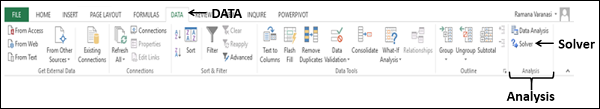
Click the DATA tab on the Ribbon. The Solver command should appear in the Analysis group as shown below.

In case you do not find the Solver command, activate it as follows −

Click the FILE tab.
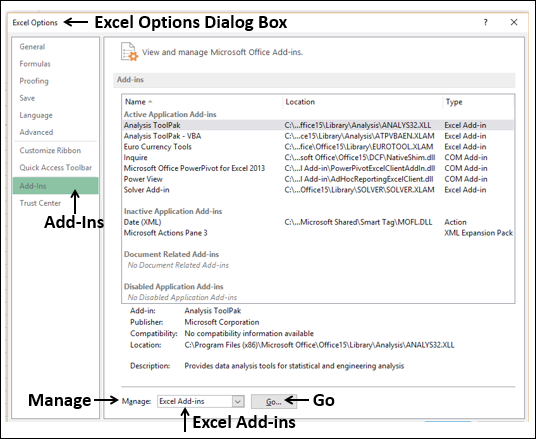
Click Options in the left pane. Excel Options dialog box appears.
Click Add-Ins in the left pane.
Select Excel Add-Ins in the Manage box and click Go.

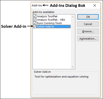
The Add-Ins dialog box appears. Check Solver Add-in and click Ok. Now, you should be able to find the Solver command on the Ribbon under the DATA tab.

Solving Methods used by Solver

You can choose one of the following three solving methods that Excel Solver supports, based on the type of problem −

LP Simplex

Used for linear problems. A Solver model is linear under the following conditions −

The target cell is computed by adding together the terms of the (changing cell)*(constant) form.
Each constraint satisfies the linear model requirement. This means that each constraint is evaluated by adding together the terms of the (changing cell)*(constant) form and comparing the sums to a constant.

Generalized Reduced Gradient (GRG) Nonlinear

Used for smooth nonlinear problems. If your target cell, any of your constraints, or both contain references to changing cells that are not of the (changing cell)*(constant) form, you have a nonlinear model.

Evolutionary

Understanding Solver Evaluation

The Solver requires the following parameters −

Decision Variable Cells
Constraint Cells
Objective Cells
Solving Method

Solver evaluation is based on the following −

The values in the decision variable cells are restricted by the values in the constraint cells.
The calculation of the value in the objective cell includes the values in the decision variable cells.
Solver uses the chosen Solving Method to result in the optimal value in the objective cell.

Defining a Problem

Suppose you are analyzing the profits made by a company that manufactures and sells a certain product. You are asked to find the amount that can be spent on advertising in the next two quarters subject to a maximum of 20,000. The level of advertising in each quarter affects the following −

The number of units sold, indirectly determining the amount of sales revenue.
The associated expenses, and
The profit.

You can proceed to define the problem as −

Find Unit Cost.
Find the advertising cost per Unit.
Find Unit Price.

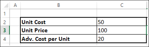
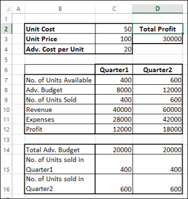
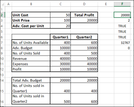
Next, set the cells for the required calculations as given below.

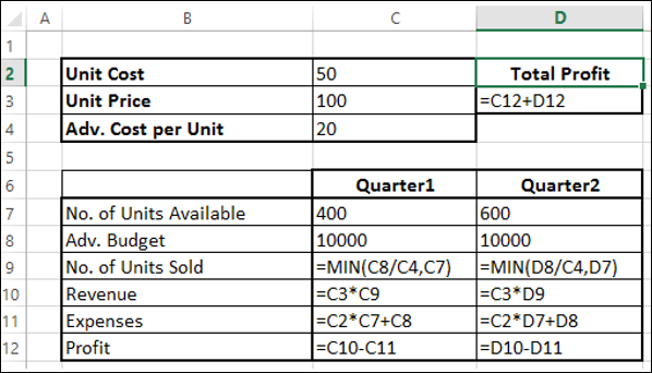
As you can observe, the calculations are done for Quarter1 and Quarter2 that are in consideration are −

No. of units available for sale in Quarter1 is 400 and in Quarter2 is 600 (cells – C7 and D7).
The initial values for advertising budget are set as 10000 per Quarter (Cells – C8 and D8).
No. of units sold is dependent on the advertising cost per unit and hence is budget for the quarter / Adv. Cost per unit. Note that we have used the Min function to take care to see that the no. of units sold in <= no. of units available. (Cells – C9 and D9).
Revenue is calculated as Unit Price * No. of Units sold (Cells – C10 and D10).
Expenses is calculated as Unit Cost * No. of Units Available + Adv. Cost for that quarter (Cells – C11 and D12).
Profit is Revenue – Expenses (Cells C12 and D12).
Total Profit is Profit in Quarter1 + Profit in Quarter2 (Cell – D3).

Next, you can set the parameters for Solver as given below −

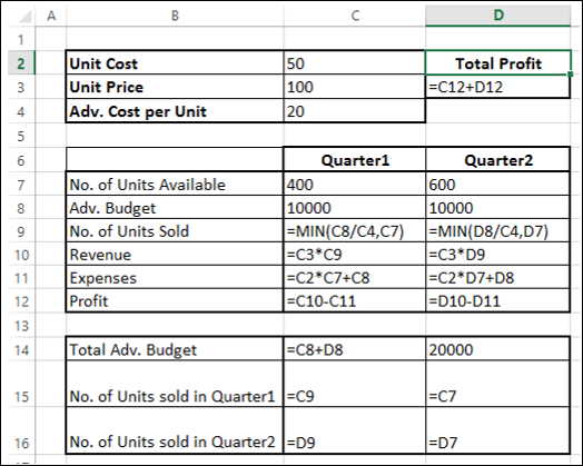
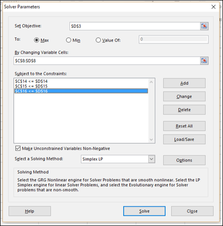
As you can observe, the parameters for Solver are −

Objective cell is D3 that contains Total Profit, which you want to maximize.
Decision Variable cells are C8 and D8 that contain the budgets for the two quarters – Quarter1 and Quarter2.
There are three Constraint cells - C14, C15 and C16.
- Cell C14 that contains total budget is to set the constraint of 20000 (cell D14).
- Cell C15 that contains the no. of units sold in Quarter1 is to set the constraint of <= no. of units available in Quarter1 (cell D15).
- Cell C16 that contains the no. of units sold in Quarter2 is to set the constraint of <= no. of units available in Quarter2 (cell D16).

Solving the Problem

The next step is to use Solver to find the solution as follows −

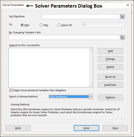
Step 1 − Go to DATA > Analysis > Solver on the Ribbon. The Solver Parameters dialog box appears.

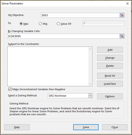
Step 2 − In the Set Objective box, select the cell D3.

Step 3 − Select Max.

Step 4 − Select range C8:D8 in the By Changing Variable Cells box.

Step 5 − Next, click the Add button to add the three constraints that you have identified.

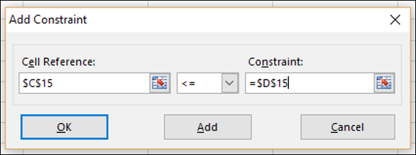
Step 6 − The Add Constraint dialog box appears. Set the constraint for total budget as given below and click Add.

Step 7 − Set the constraint for total no. of units sold in Quarter1 as given below and click Add.

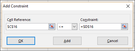
Step 8 − Set the constraint for total no. of units sold in Quarter2 as given below and click OK.

The Solver Parameters dialog box appears with the three constraints added in box –Subject to the Constraints.

Step 9 − In the Select a Solving Method box, select Simplex LP.

Step 10 − Click the Solve button. The Solver Results dialog box appears. Select Keep Solver Solution and click OK.

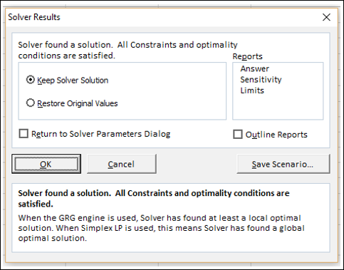
The results will appear in your worksheet.

As you can observe, the optimal solution that produces maximum total profit, subject to the given constraints, is found to be the following −

Total Profit – 30000.
Adv. Budget for Quarter1 – 8000.
Adv. Budget for Quarter2 – 12000.

Stepping through Solver Trial Solutions

You can step through the Solver trial solutions, looking at the iteration results.

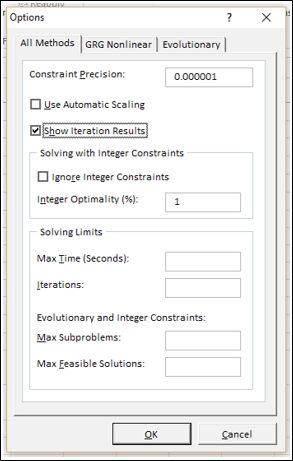
Step 1 − Click the Options button in the Solver Parameters dialog box.

The Options dialog box appears.

Step 2 − Select the Show Iteration Results box and click OK.

Step 3 − The Solver Parameters dialog box appears. Click Solve.

Step 4 − The Show Trial Solution dialog box appears, displaying the message - Solver paused, current solution values displayed on worksheet.

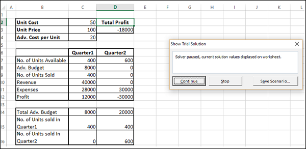
As you can observe, the current iteration values are displayed in your working cells. You can either stop the Solver accepting the current results or continue with the Solver from finding solution in further steps.

Step 5 − Click Continue.

The Show Trial Solution dialog box appears at every step and finally after the optimal solution is found, Solver Results dialog box appears. Your worksheet is updated at every step, finally showing the result values.

Saving Solver Selections

You have the following saving options for the problems that you solve with Solver −

You can save the last selections in the Solver Parameters dialog box with a worksheet by saving the workbook.
Each worksheet in a workbook can have its own Solver selections, and all of them will be saved when you save the workbook.
You can also define more than one problem in a worksheet, each with its own Solver selections. In such a case, you can load and save problems individually with the Load/Save in the Solver Parameters dialog box.
- Click the Load/Save button. The Load/Save dialog box appears.
- To save a problem model, enter the reference for the first cell of a vertical range of empty cells in which you want to place the problem model. Click Save.

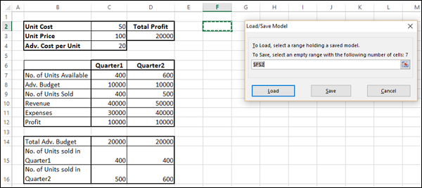
The problem model (the Solver Parameters set) appears starting at the cell that you have given as the reference.

To load a problem model, enter the reference for the entire range of cells that contains the problem model. Then, click on the Load button.