- Excel Data Analysis - Home
- Data Analysis - Overview
- Data Analysis - Process
- Excel Data Analysis - Overview
- Working with Range Names
- Tables
- Cleaning Data with Text Functions
- Cleaning Data Contains Date Values
- Working with Time Values
- Conditional Formatting
- Sorting
- Filtering
- Subtotals with Ranges
- Quick Analysis
- Lookup Functions
- PivotTables
- Data Visualization
- Data Validation
- Financial Analysis
- Working with Multiple Sheets
- Formula Auditing
- Inquire
- Advanced Data Analysis - Overview
- Data Consolidation
- What-If Analysis
- What-If Analysis with Data Tables
- What-If Analysis Scenario Manager
- What-If Analysis with Goal Seek
- Optimization with Excel Solver
- Importing Data into Excel
- Data Model
- Exploring Data with PivotTables
- Exploring Data with Powerpivot
- Exploring Data with Power View
- Exploring Data Power View Charts
- Exploring Data Power View Maps
- Exploring Data PowerView Multiples
- Exploring Data Power View Tiles
- Exploring Data with Hierarchies
- Aesthetic Power View Reports
- Key Performance Indicators
- Excel Data Analysis Resources
- Excel Data Analysis - Quick Guide
- Excel Data Analysis - Resources
- Excel Data Analysis - Discussion
Excel Data Analysis - Lookup Functions
You can use Excel functions to −
- Find values in a range of data - VLOOKUP and HLOOKUP
- Obtain a value or the reference to a value from within a table or range - INDEX
- Obtain the relative position of a specified item in a range of cells - MATCH
You can also combine these functions to get the required results based on the inputs you have.
Using VLOOKUP Function
The syntax of the VLOOKUP function is
VLOOKUP (lookup_value, table_array, col_index_num, [range_lookup])
Where
lookup_value − is the value you want to look up. Lookup_value can be a value or a reference to a cell. Lookup_value must be in the first column of the range of cells you specify in table_array
table_array − is the range of cells in which the VLOOKUP will search for the lookup_value and the return value. table_array must contain
the lookup_value in the first column, and
the return value you want to find
Note − The first column containing the lookup_value can either be sorted in ascending order or not. However, the result will be based on the order of this column.
col_index_num − is the column number in the table_array that contains the return value. The numbers start with 1 for the left-most column of table-array
range_lookup − is an optional logical value that specifies whether you want VLOOKUP to find an exact match or an approximate match. range_lookup can be
omitted, in which case it is assumed to be TRUE and VLOOKUP tries to find an approximate match
TRUE, in which case VLOOKUP tries to find an approximate match. In other words, if an exact match is not found, the next largest value that is less than lookup_value is returned
FALSE, in which case VLOOKUP tries to find an exact match
1, in which case it is assumed to be TRUE and VLOOKUP tries to find an approximate match
0, in which case it is assumed to be FALSE and VLOOKUP tries to find an exact match
Note − If range_lookup is omitted or TRUE or 1, VLOOKUP works correctly only when the first column in table_array is sorted in ascending order. Otherwise, it may result in incorrect values. In such a case, use FALSE for range_lookup.
Using VLOOKUP Function with range_lookup TRUE
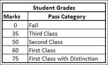
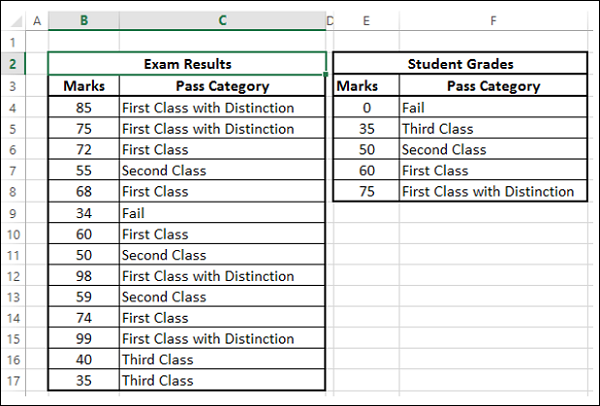
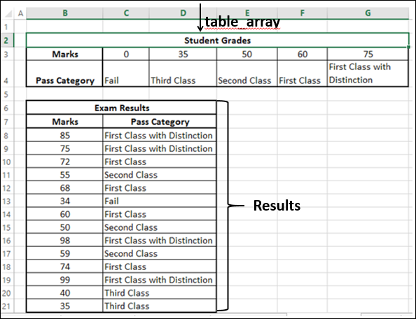
Consider a list of student marks. You can obtain the corresponding grades with VLOOKUP from an array containing the marks intervals and pass category.
table_array −
Note that the first column marks based on which the grades are obtained is sorted in ascending order. Hence, using TRUE for range_lookup argument you can get approximate match that is what is required.
Name this array as Grades.
It is a good practice to name arrays in this way so that you need not remember the cell ranges. Now, you are ready to look up the grade for the list of marks you have as follows −
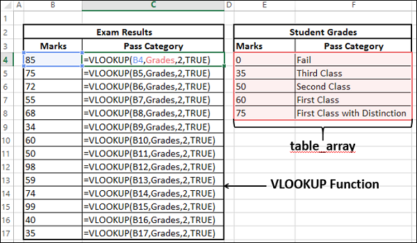
As you can observe,
col_index_num − indicates the column of the return value in table_array is 2
the range_lookup is TRUE
The first column containing the lookup value in the table_array grades is in ascending order. Hence, the results will be correct.
You can get the return value for approximate matches also. i.e. VLOOKUP computes as follows −
| Marks | Pass Category |
|---|---|
| < 35 | Fail |
| >= 35 and < 50 | Third Class |
| >= 50 and < 60 | Second Class |
| >=60 and < 75 | First Class |
| >= 75 | First Class with Distinction |
You will get the following results −
Using VLOOKUP Function with range_lookup FALSE
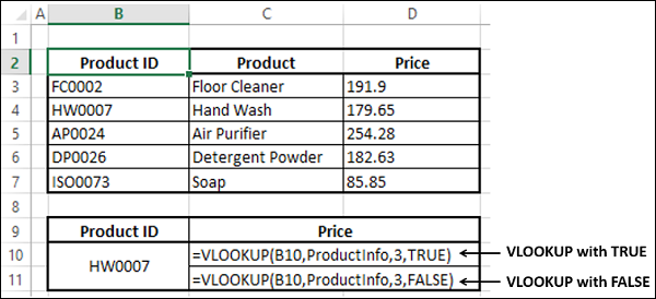
Consider a list of products containing the Product ID and price for each of the products. The product ID and price will be added to the end of the list whenever a new product is launched. This would mean that the product IDs need not be in ascending order. The product list might be as shown below −
table_array −
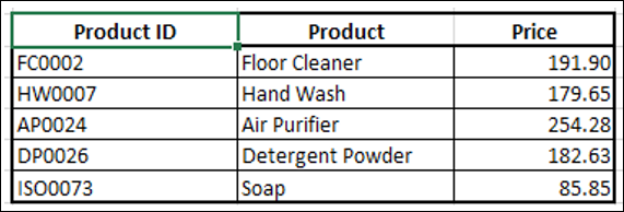
Name this array as ProductInfo.
You can obtain the price of a product given the product ID with the VLOOKUP function as the product ID is in the first column. The price is in column 3 and hence col_index_ num should be 3.
- Use VLOOKUP Function with range_lookup as TRUE
- Use VLOOKUP Function with range_lookup as FALSE
The correct answer is from the ProductInfo array is 171.65. You can check the results.
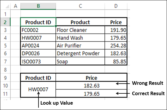
You observe that you got −
- The correct result when range_lookup is FALSE, and
- A wrong result when range_lookup is TRUE.
This is because, the first column in the ProductInfo array is not sorted in ascending order. Hence, remember to use FALSE whenever the data is not sorted.
Using HLOOKUP Function
You can use HLOOKUP function if the data is in rows rather than columns.
Example
Let us take the example of product information. Suppose the array looks as follows −
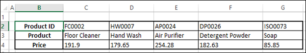
Name this Array ProductRange. You can find the price of a product given the product ID with HLOOKUP function.
The Syntax of HLOOKUP function is
HLOOKUP (lookup_value, table_array, row_index_num, [range_lookup])
Where
lookup_value − is the value to be found in the first row of the table
table_array − is a table of information in which data is looked up
row_index_num − is the row number in table_array from which the matching value will be returned
range_lookup − is a logical value that specifies whether you want HLOOKUP to find an exact match or an approximate match
range_lookup can be
omitted, in which case it is assumed to be TRUE and HLOOKUP tries to find an approximate match
TRUE, in which case HLOOKUP tries to find an approximate match. In other words, if an exact match is not found, the next largest value that is less than lookup_value is returned
FALSE, in which case HLOOKUP tries to find an exact match
1, in which case it is assumed to be TRUE and HLOOKUP tries to find an approximate match
0, in which case it is assumed to be FALSE and HLOOKUP tries to find an exact match
Note − If range_lookup is Omitted or TRUE or 1, HLOOKUP works correctly only when the first column in table_array is sorted in ascending order. Otherwise, it may result in incorrect values. In such a case, use FALSE for range_lookup.
Using HLOOKUP Function with range_lookup FALSE
You can obtain the price of a product given the product ID with the HLOOKUP function as the product ID is in the first row. The price is in row 3 and hence row_index_ num should be 3.
- Use HLOOKUP Function with range_lookup as TRUE.
- Use HLOOKUP Function with range_lookup as FALSE.
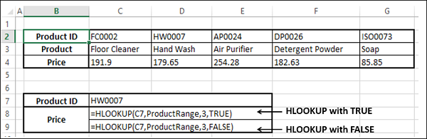
The correct answer from the ProductRange array is 171.65. You can check the results.
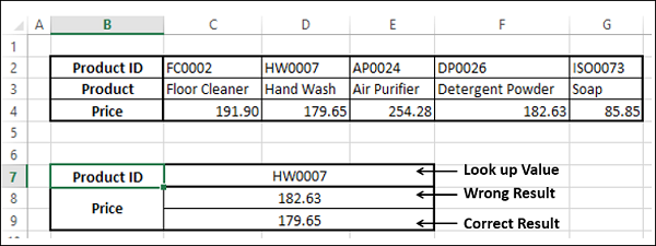
You observe that as in the case of VLOOKUP, you got
The correct result when range_lookup is FALSE, and
A wrong result when range_lookup is TRUE.
This is because the first row in the ProductRange array is not sorted in ascending order. Hence, remember to use FALSE whenever the data is not sorted.
Using HLOOKUP Function with range_lookup TRUE
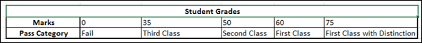
Consider the example of student marks used in VLOOKUP. Suppose you have the data in rows instead of columns as shown in the table given below −
table_array −
Name this array as GradesRange.
Note that the first row marks based on which the grades are obtained is sorted in ascending order. Hence, using HLOOKUP with TRUE for range_lookup argument, you can get the Grades with approximate match and that is what is required.
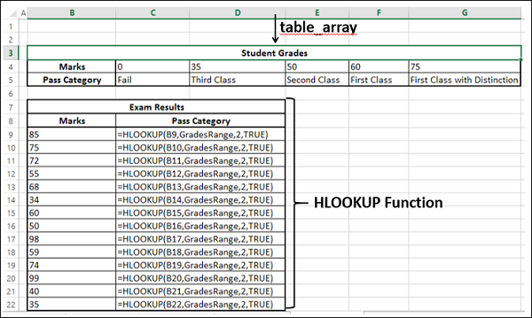
As you can observe,
row_index_num − indicates the column of the return value in table_array is 2
the range_lookup is TRUE
The first column containing the lookup value in the table_array Grades is in ascending order. Hence, the results will be correct.
You can get the return value for approximate matches also. i.e. HLOOKUP computes as follows −
| Marks | < 35 | >= 35 and < 50 | >= 50 and < 60 | >=60 and < 75 | >= 75 |
|---|---|---|---|---|---|
| Pass Category | Fail | Third Class | Second Class | First Class | First Class with Distinction |
You will get the following results −
Using INDEX Function
When you have an array of data, you can retrieve a value in the array by specifying the row number and column number of that value in the array.
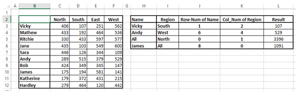
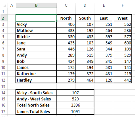
Consider the following sales data, wherein you find the sales in each of the North, South, East and West regions by the salespersons who are listed.
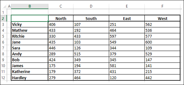
- Name the array as SalesData.
Using INDEX Function, you can find −
- The Sales of any of the Salespersons in a certain Region.
- Total Sales in a Region by all the Salespersons.
- Total Sales by a Salesperson in all the Regions.
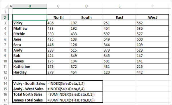
You will get the following results −
Suppose you do not know the row numbers for the salespersons and column numbers for the regions. Then, you need to find the row number and column number first before you retrieve the value with the index function.
You can do it with the MATCH function as explained in the next section.
Using MATCH Function
If you need the position of an item in a range, you can use the MATCH function. You can combine MATCH and INDEX functions as follows −
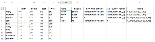
You will get the following results −