Excel Data Analysis - Filtering

---

---

Filtering allows you to extract data that meets the defined criteria from a given Range or table. This is a quick way to display only the information that is needed by you.

You can Filter data in a Range, table or PivotTable.

You can filter data by −

• Selected values
• Text filters if the column you selected contains text
• Date filters if the column you selected contains dates
• Number filters if the column you selected contains numbers
• Number filters if the column you selected contains numbers
• Font color if the column you selected contains font with color
• Cell icon if the column you selected contains cell icons
• Advanced filter
• Using slicers

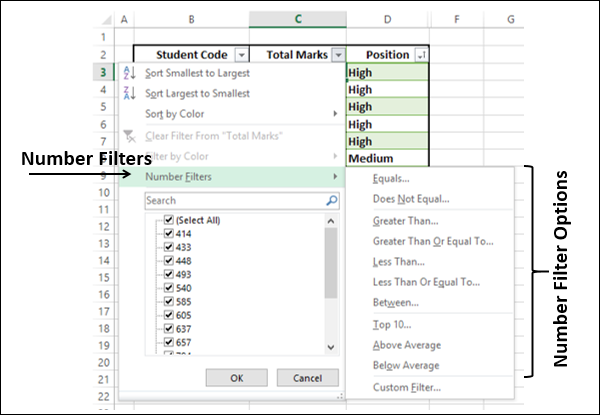
In a table, the column headers are automatically tagged to filters, known as AutoFilters. AutoFilter is represented by the arrow next to column header. Each AutoFilter has filter options based on the type of data you have in that column. For example, if the column contains numbers, when you click on the arrow next to the column header, Number Filter Options appear.

When you click a Filter option or when you click on Custom Filter that appears at the end of the Filter options, Custom AutoFilter dialog box appears, wherein you can customize your filtering options.

In case of a Range, you can provide the column headers in the first row of the range and click on filter in the Editing group on Home tab. This will make the AutoFilter on for the Range. You can remove the filters that you have in your data. You can also reapply the filters when data changes occur.

Filter by Selected Values

You can choose what data is to be displayed by clicking the arrow next to a column header and selecting the Values in the column. Only those rows containing the selected values in the chosen column will be displayed.

Consider the following data −

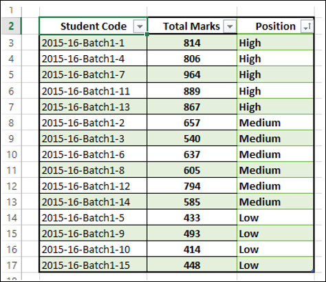
If you want to display the data only for Position = High, click the arrow next to Position. A drop-down box appears with all the values in the position column. By default, all the values will be selected.

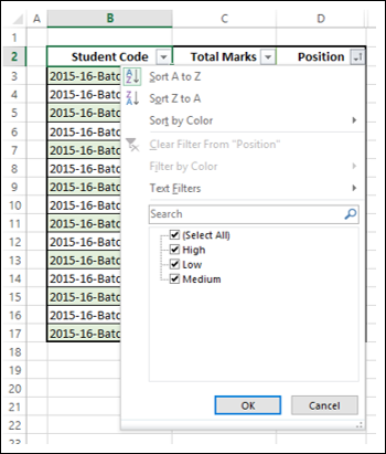
• Click Select All. All the boxes are cleared.
• Select High as shown in the following screen shot.

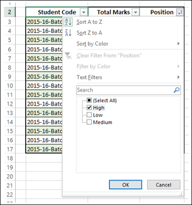
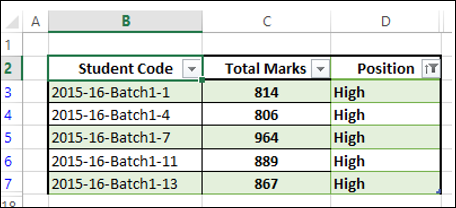
Click OK. Only those Rows, which have the value High as Position, will be displayed.

Filter by Text

Consider the following data −

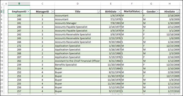
You can filter this data such that only those Rows wherein the Title is “Manager” will be displayed.

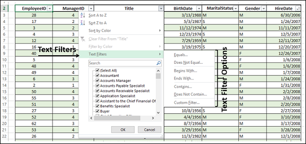
Click the arrow next to the column header Title. From the drop-down list, click Text Filters. Text filter options appear.

Select Contains from the available options. The Custom AutoFilter dialog box opens. Type Manager in the Box next to Contains.

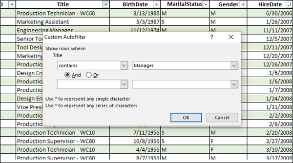
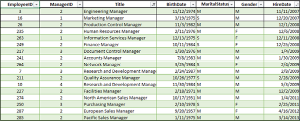
Click OK. Only the Rows where Title contains Manager will be displayed.

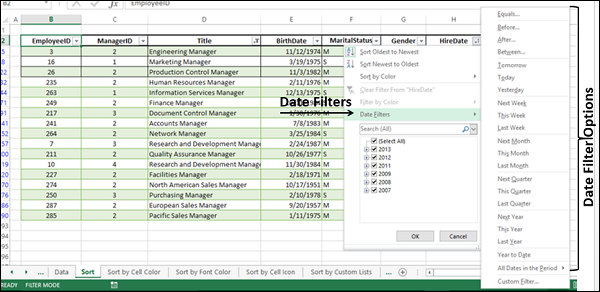
Filter by Date

You can filter this data further such that only those Rows wherein the Title is “Manager” and HireDate is prior to 2011 can be displayed. That means you will display the Employee information for all the managers who have been with the organization from before 2011.

Click the arrow next to the column header HireDate. From the drop-down list, click Date Filters. The Date filter options appear. Select Before from the drop-down list.

Custom AutoFilter dialog box opens. Type 1/1/2011 in the box next to is before. You can also select the date from the date picker next to the box.

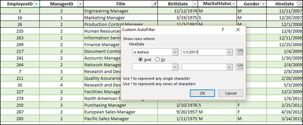
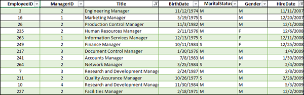
Click OK. Only the rows where Title contains Manager and HireDate is prior to 1/1/2011 will be displayed.

Filter by Numbers

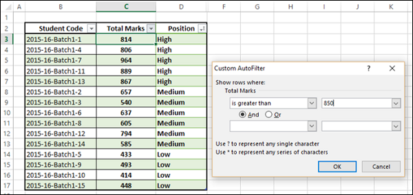
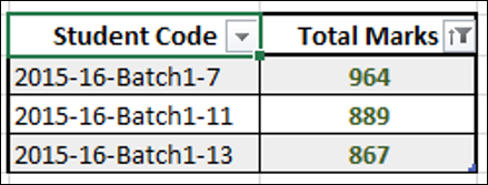
Consider the following data −

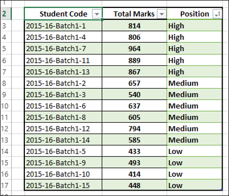
You can filter this data such that only those rows where Total Marks > 850 can be displayed.

Click the arrow next to the column header Total Marks. From the drop-down list, click Number Filters. The Number Filter options appear.

Click Greater Than. Custom AutoFilter dialog box opens. Type 850 in the box next to Greater Than.

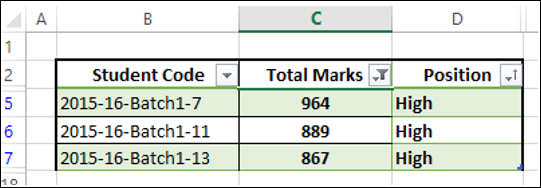
Click OK. Only the rows wherein the total marks are greater than 850 will be displayed.

Filter by Cell Color

If the data has different cell colors or is conditionally formatted, you can filter by the colors that are displayed in your table.

Consider the following data. The column Total Marks has conditional formatting with different cell colors.

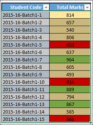
Click the arrow in the header Total Marks. From the drop-down list, click Filter by Color. The Filter by Cell Color options appear.

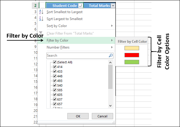
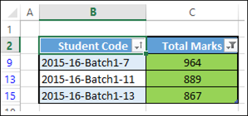
Select the green color and click OK. Only the rows wherein the total marks column has green color cells will be displayed.

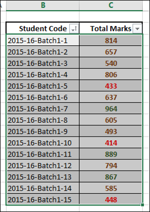
Filter by Font Color

If the data has different font colors or is conditionally formatted, you can filter by the colors that are displayed in your table.

Consider the following data. The column - Total Marks has conditional formatting with font color applied.

Click the arrow in the header Total Marks. From the Drop-Down List, click Filter by Color. Filter by Font Color options appear.

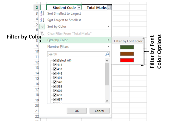
Select the green color and click OK. Only the rows wherein the Total Marks column has green color font will be displayed.

Filter by Cell Icon

If the data has different icons or a conditional format, you can filter by the icons that are shown in your table.

Consider the following data. The column Total Marks has conditional formatting with icons applied.

Click the arrow in the header Total Marks. From the drop-down list, select Filter by Color. The Filter by Cell Icon options appear.

Select the icon and click OK.

Only the rows wherein the Total Marks column has the icon will be displayed.

Clear Filter

Removing filters is termed as Clear Filter in Excel.

You can remove

• A filter from a specific column, or
• All of the filters in the worksheet at once.

To remove a filter from a specific column, click the arrow in the table header of that column. From the drop-drown menu, click Clear Filter From “<specific Column Name>”.

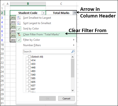
The filter in the column is removed. To remove filtering from the entire worksheet, select Clear in the

• Editing group on the Home tab, or

• Sort & Filter group in the Data tab.

All the filters in the worksheet are removed at once. Click Undo Show All if you have removed the Filters by mistake.

Reapply Filter

When changes occur in your data, click Reapply in Sort & Filter group on the Data tab. The defined filter will be applied again on the modified data.

Advanced Filtering

You can use Advance Filtering if you want to filter the data of more than one column.

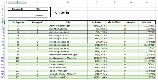
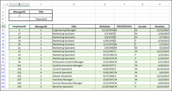
You need to define your filtering criteria as a range. Suppose you want to display the information of those employees who are specialists or whose EmployeeID is 2, define the Criteria as follows −

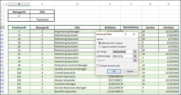
• Next, click Advanced in the Sort & Filter group on the Data tab. The Advanced Filter dialog box appears.

• Specify the List Range and the Criteria Range.

• You can either filter the list, in place or copy to another location.

• In the filtering given below, filter the data in place is chosen.

The employee information where ManagerID = 2 OR Title = “*Specialist” is displayed.

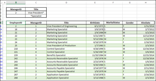
Suppose you want to display information about specialists and vice presidents. You can define the criteria and filter as follows −

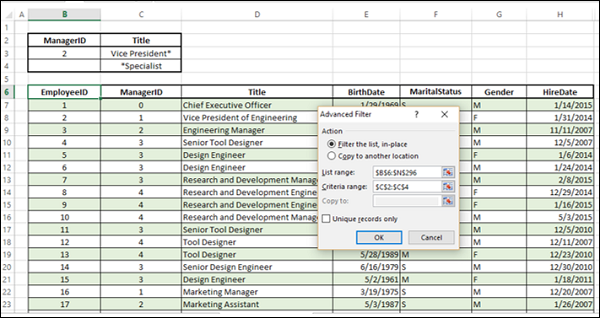
The criteria you applied is Title = “*Specialist” OR Title = “Vice President”. The employee information of specialists and vice presidents will be displayed.

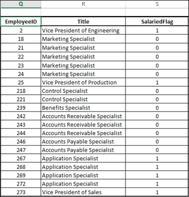
You can copy the filtered data to another location. You can also select only few columns to include in the copy operation.

• Copy EmployeedID, Title and SalariedFlag to the Cells Q2, R2, S2. This will be the first Row of your filtered data.

• Click on Advanced and in the Advanced Filter dialog box, click on Copy to another location. In the Copy to box, specify reference to the Headers you copied in another location, i.e. Q2:S2.

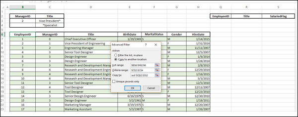
Click OK after specifying the List Range and Criteria Range. The selected columns in the filtered data will be copied to the location you specified.

Filter Using Slicers

Slicers to filter data in PivotTables were introduced in Excel 2010. In Excel 2013, you can use Slicers to filter data in tables also.

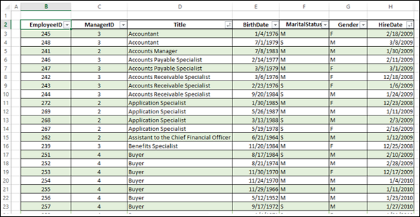
Consider the data in the following table.

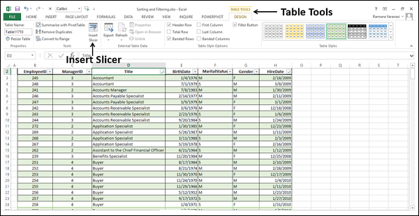
• Click the Table.
• Click Table Toolsthat appear on the Ribbon.
• The Design Ribbon appears.
• Click Insert Slicer.

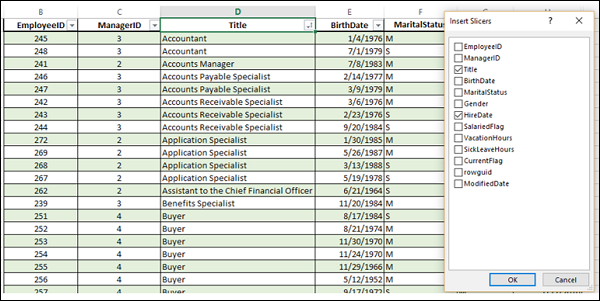
• Insert Slicers dialog box appears as shown in the screen shot given below.

• In the Insert Slicers dialog box, you will find all the column headers including those columns that are hidden.

• Check the boxes Title and HireDate. Click OK.

A Slicer appears for each of the table headers you checked in the Insert Slicers dialog box. In each Slicer, all the values of that column will be highlighted.

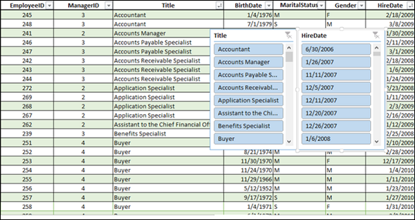
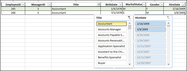
In the Title Slicer, click the first value. Only that value will be highlighted and the rest of the values get unselected. Further, you will find the values in HireDate Slicer that are corresponding to the value in the Title Slicer also get highlighted.

In the table, only the selected values are displayed.

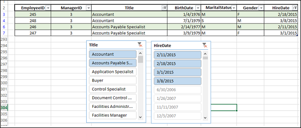
You can select / deselect the values in the Slicers and you find that the data is automatically updated in the table. To choose more than one value, hold down the Ctrl key, and pick the values that you want to display.

Select the Title values that belong to the Accounts department and the HireDate values in the year 2015 from the two Slicers.

You can clear the selections in any Slicer by clicking the Clear Filter at the right end corner of the Slicer header.