Kibana - Aggregation And Metrics

---

The two terms that you come across frequently during your learning of Kibana are Bucket and Metrics Aggregation. This chapter discusses what role they play in Kibana and more details about them.

What is Kibana Aggregation?

Aggregation refers to the collection of documents or a set of documents obtained from a particular search query or filter. Aggregation forms the main concept to build the desired visualization in Kibana.

Whenever you perform any visualization, you need to decide the criteria, which means in which way you want to group the data to perform the metric on it.

In this section, we will discuss two types of Aggregation −

• Bucket Aggregation
• Metric Aggregation

Bucket Aggregation

A bucket mainly consists of a key and a document. When the aggregation is executed, the documents are placed in the respective bucket. So at the end you should have a list of buckets, each with a list of documents. The list of Bucket Aggregation you will see while creating visualization in Kibana is shown below −

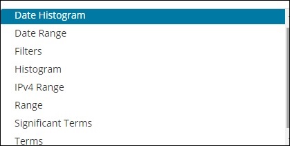
Bucket Aggregation has the following list −

• Date Histogram
• Date Range
• Filters
• Histogram
• IPv4 Range
• Range
• Significant Terms
• Terms

While creating, you need to decide one of them for Bucket Aggregation i.e. to group the documents inside the buckets.

As an example, for analysis, consider the countries data that we have uploaded at the start of this tutorial. The fields available in the countries index is country name, area, population, region. In the countries data, we have name of the country along with its population, region and the area.

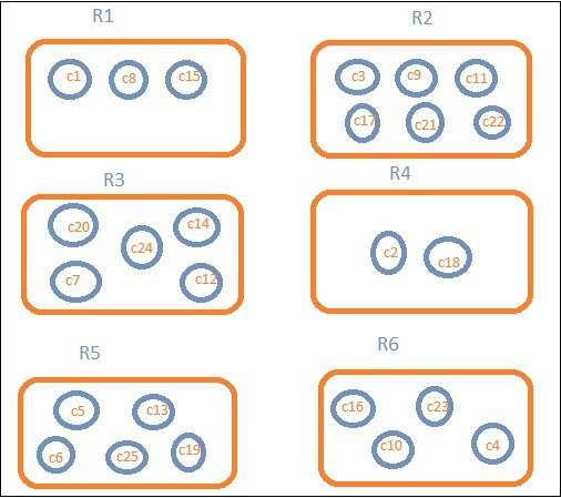
Let us assume that we want region wise data. Then, the countries available in each region becomes our search query, so in this case the region will form our buckets. The block diagram below shows that R1, R2,R3,R4,R5 and R6 are the buckets which we got and c1 , c2 ..c25 are the list of documents which are part of the buckets R1 to R6.

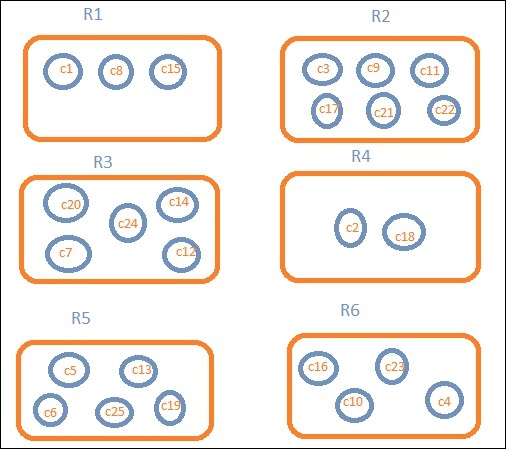
We can see that there are some circles in each of the bucket. They are set of documents based on the search criteria and considered to be falling in each of the bucket. In the bucket R1, we have documents c1, c8 and c15. These documents are the countries that falling in that region, same for others. So if we count the countries in Bucket R1 it is 3, 6 for R2, 6 for R3, 2 for R4, 5 for R5 and 4 for R6.

So through bucket aggregation, we can aggregate the document in buckets and have a list of documents in those buckets as shown above.

The list of Bucket Aggregation we have so far is −

• Date Histogram
• Date Range
• Filters
• Histogram
• IPv4 Range
• Range
• Significant Terms
• Terms

Let us now discuss how to form these buckets one by one in detail.

Date Histogram

Date Histogram aggregation is used on a date field. So the index that you use to visualize, if you have date field in that index than only this aggregation type can be used. This is a multi-bucket aggregation which means you can have some of the documents as a part of more than 1 bucket. There is an interval to be used for this aggregation and the details are as shown below −

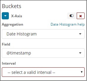
When you Select Buckets Aggregation as Date Histogram, it will display the Field option which will give only the date related fields. Once you select your field, you need to select the Interval which has the following details −

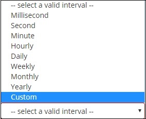
So the documents from the index chosen and based on the field and interval chosen will categorize the documents in buckets. For example, if you chose the interval as monthly, the documents based on date will be converted into buckets and based on the month i.e, Jan-Dec the documents will be put in the buckets. Here Jan,Feb,..Dec will be the buckets.

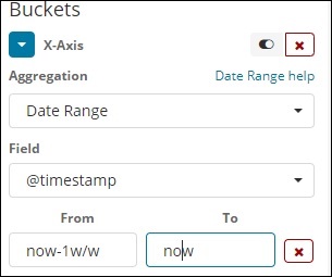
Date Range

You need a date field to use this aggregation type. Here we will have a date range, that is from date and to date are to be given. The buckets will have its documents based on the form and to date given.

Filters

With Filters type aggregation, the buckets will be formed based on the filter. Here you will get a multi-bucket formed as based on the filter criteria one document can exists in one or more buckets.

Using filters, users can write their queries in the filter option as shown below −

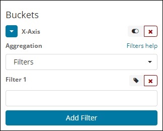
You can add multiple filters of your choice by using Add Filter button.

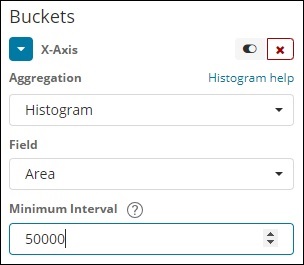
Histogram

This type of aggregation is applied on a number field and it will group the documents in a bucket based on the interval applied. For example, 0-50,50-100,100-150 etc.

IPv4 Range

This type of aggregation is used and mainly used for IP addresses.

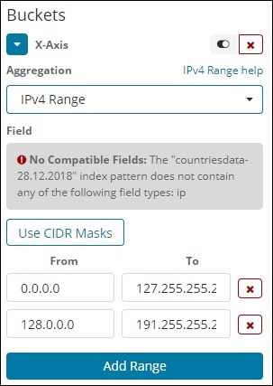
The index that we have that is the contriesdata-28.12.2018 does not have field of type IP so it displays a message as shown above. If you happen to have the IP field, you can specify the From and To values in it as shown above.

Range

This type of Aggregation needs fields to be of type number. You need to specify the range and the documents will be listed in the buckets falling in the range.

You can add more range if required by clicking on the Add Range button.

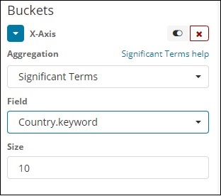
Significant Terms

This type of aggregation is mostly used on the string fields.

Terms

This type of aggregation is used on all the available fields namely number, string, date, boolean, IP address, timestamp etc. Note that this is the aggregation we are going to use in all our visualization that we are going to work on in this tutorial.

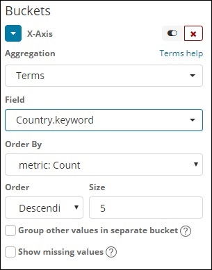
We have an option order by which we will group the data based on the metric we select. The size refers to the number of buckets you want to display in the visualization.

Next, let us talk about Metric Aggregation.

Metric Aggregation

Metric Aggregation mainly refers to the maths calculation done on the documents present in the bucket. For example if you choose a number field the metric calculation you can do on it is COUNT, SUM, MIN, MAX, AVERAGE etc.

A list of metric aggregation that we shall discuss is given here −

In this section, let us discuss the important ones which we are going to use often −

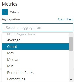
• Average
• Count
• Max
• Min
• Sum

The metric will be applied on the individual bucket aggregation that we have already discussed above.

Next, let us discuss the list of metrics aggregation here −

Average

This will give the average for the values of the documents present in the buckets. For example −

R1 to R6 are the buckets. In R1 we have c1,c8 and c15. Consider the value of c1 is 300, c8 is500 and c15 is 700. Now to get the average value of R1 bucket

R1 = value of c1 + value of c8 + value of c15 / 3 = 300 + 500 + 700 / 3 = 500.

The average is 500 for bucket R1. Here the value of the document could be anything like if you consider the countries data it could be the area of the country in that region.

Count

This will give the count of documents present in the Bucket. Suppose you want the count of the countries present in the region, it will be the total documents present in the buckets. For example, R1 it will be 3, R2 = 6, R3 = 5, R4 = 2, R5 = 5 and R6 = 4.

Max

This will give the max value of the document present in the bucket. Considering the above example if we have area wise countries data in the region bucket. The max for each region will be the country with the max area. So it will have one country from each region i.e. R1 to R6.

in

This will give the min value of the document present in the bucket. Considering above example if we have area wise countries data in the region bucket. The min for each region will be the country with the minimum area. So it will have one country from each region i.e. R1 to R6.

Sum

This will give the sum of the values of the document present in the bucket. For example if you consider the above example if we want the total area or countries in the region, it will be sum of the documents present in the region.

For example, to know the total countries in the region R1 it will be 3, R2 = 6, R3 = 5, R4 = 2, R5 = 5 and R6 = 4.

In case we have documents with area in the region than R1 to R6 will have the country wise area summed up for the region.