How to make a pictograph (chart with pictures) in Excel?

In this article, we will describe the method to make a pictograph in Excel. Excel is a software application that focuses on numeric data. To analyze numeric data more effectively and efficiently, Excel provides a way to visualize this numeric data in the form of charts and plots. Excel provides functionalities to develop many kinds of charts and plots. A pictograph is one such chart that contains pictures. A pictograph can be defined as a chart with pictures or icons.

Let us see how to make a pictograph in Excel.

Example

The following steps need to be implemented to create a pictograph using Excel.

Step 1

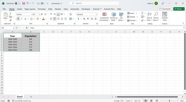
Create a dataset. In our example, we are creating a dataset for the world population over the years. This dataset contains the world population starting from the year 2000 and records the population in lakhs every five years.

The dataset is as follows

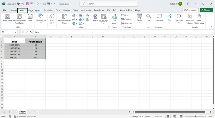
Step 2

Choose the data and then click on the tab named Insert.

Step 3

Under the Insert tab, click on Charts as highlighted in the below figure −

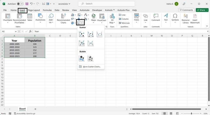
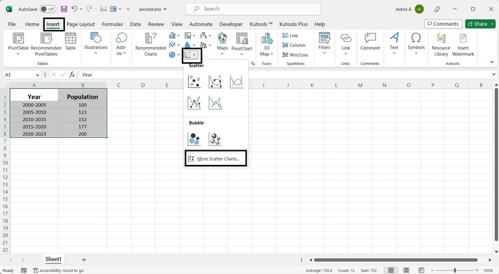
Step 4

Clicking on Charts will display various designs of scatter plots. But we need a Bar Chart hence we click on the arrow under the heading More Scatter Charts.

Step 5

A box will appear with all the available options for charts and plots on the left side. Click on Bar Chart. You can select any bar chart design of your choice. After this, click on the OK button.

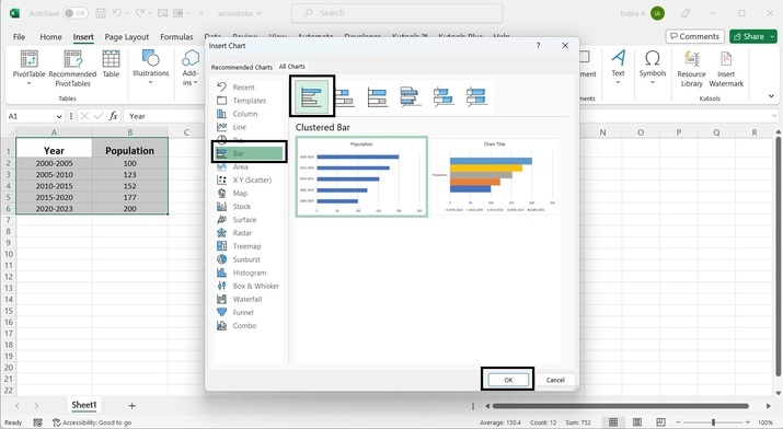
A bar chart will appear on the current worksheet as shown.

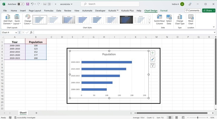
Step 6

Click on the bars in the bar chart.

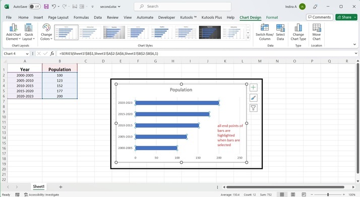
Note − When the bars are selected, the endpoints of the bars are highlighted with small circles as shown in the above image.

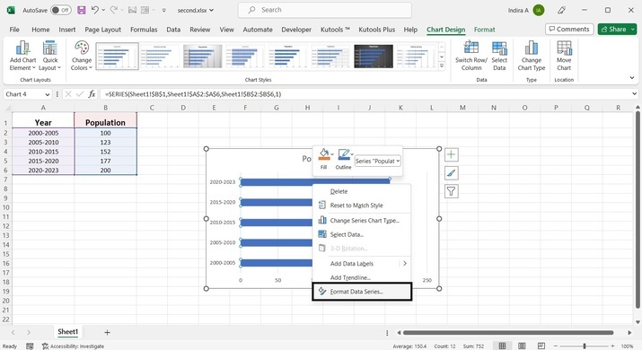
Step 7

Right-click and select the last option which is Format Data Series. A pane will appear on the right side of the worksheet. This pane will have the heading Format Data Series.

Step 8

Click on the first icon which is the Fill option. Then check Picture or Texture fill radio button.

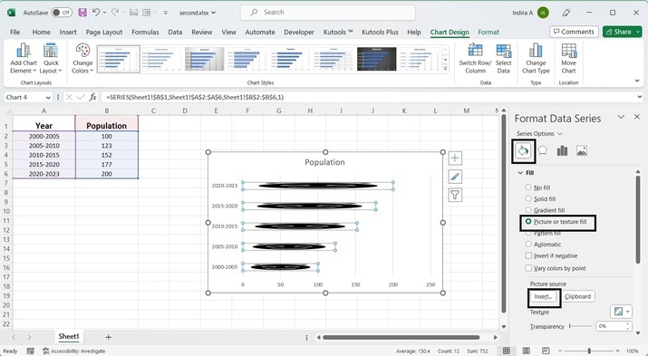
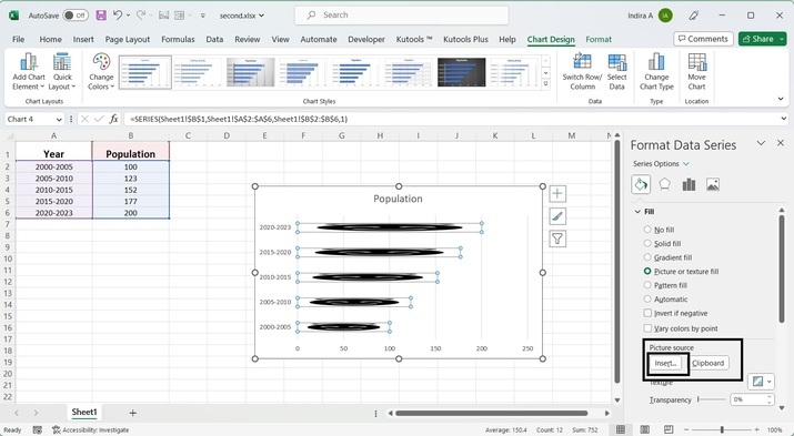
Step 9

Under the Picture Source heading, click on the Insert button. A box will appear will four options.

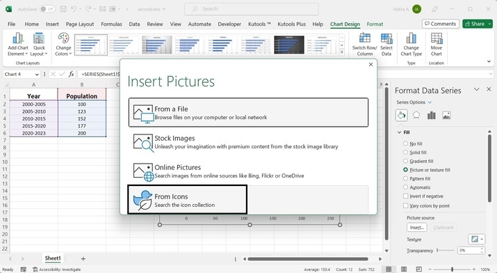
Step 10

Click on the last option which is the From Icons option.

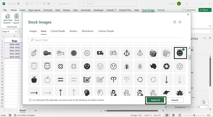
Select an icon from the given collection of icons. Then click on the Insert button.

Step 11

Select Stack on the pane as shown. The bars in the bar chart will be replaced with the selected icons.

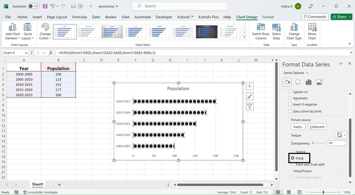
As seen from the output image, the bars in the bar charts are replaced by the icon which is selected.

Note − This article references Excel from Microsoft 365 suite. The options under the Charts heading can vary with different versions of Excel. It is better to go through all the options under the Charts heading and then select the option to create a bar chart.

Conclusion

This article describes the method to create a pictograph in Excel. It is recommended that the users should be well-versed in the method of creating charts and plots in Excel. If not, it is required that the user should first get comfortable with charts in Excel and only then proceed with the method outlined in this article.