How to add a scrollbar to a chart in Excel

MS Excel Microsoft Technologies Advanced Excel Function

You can use the scrollbar feature to show a chart with lots of data, just by dragging the scrollbar, you will see the data changing continuously while it's being displayed in the chart. If a lot of data needs to be shown, you can add the scrollbar. However, there is a tricky part in Excel when it comes to adding a scrollbar to a chart, so follow these steps step by step to finish this task.

Add a Scrollbar in Excel

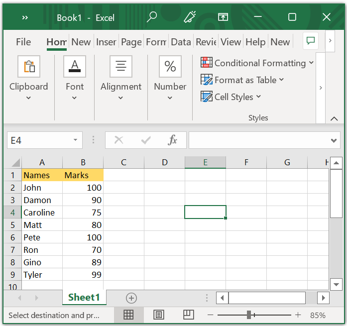
You have the following data range wherein you want to add the scrollbar chart to the Excel worksheet.

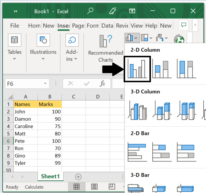
Step 1

The first thing you can do is insert a chart with the above data by selecting the data and then clicking Insert > Column > Clustered Column.

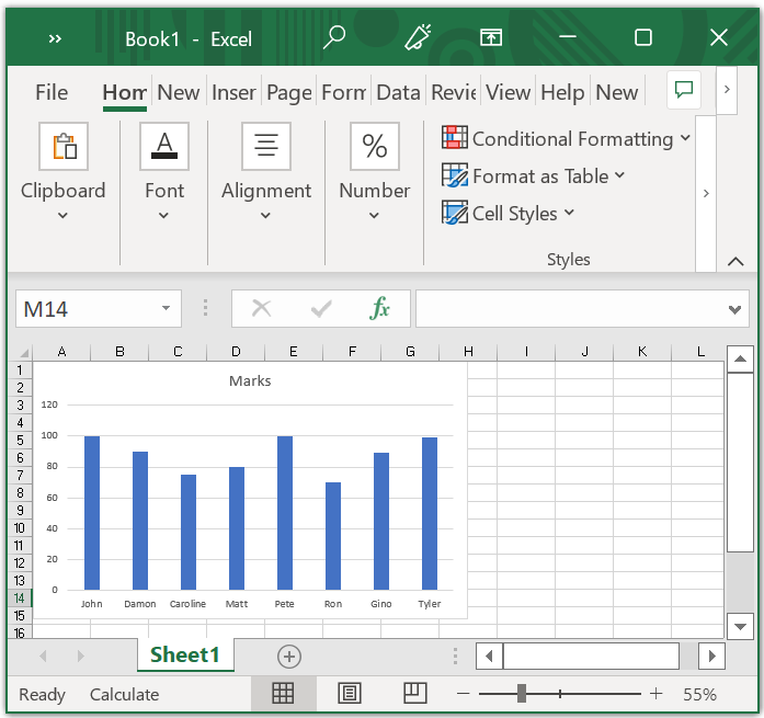
Step 2

Column chart will get inserted into your Excel Workbook.

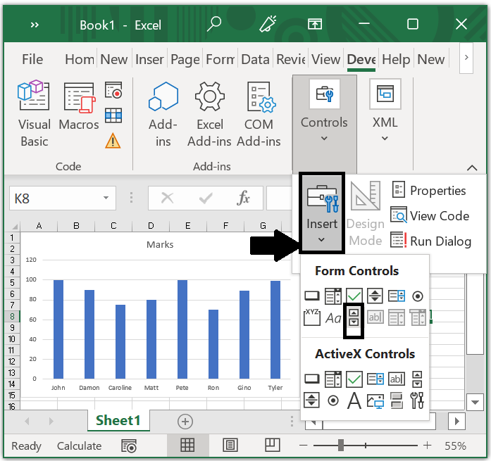
Step 3

Now you need to insert the scrollbar into the Excel workbook, to do this go to Developer > Insert > Scrollbar.

Note

You can display the Developer tab on the ribbon by clicking File > Option > Customize Ribbon, and in the right section, you can check Developer to display it on the ribbon when the Developer tab is not visible on ribbon.

Step 4

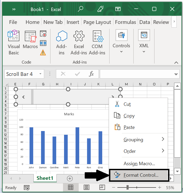
After this drag the mouse to draw a scrollbar and right-click to select Format Control.

Step 5

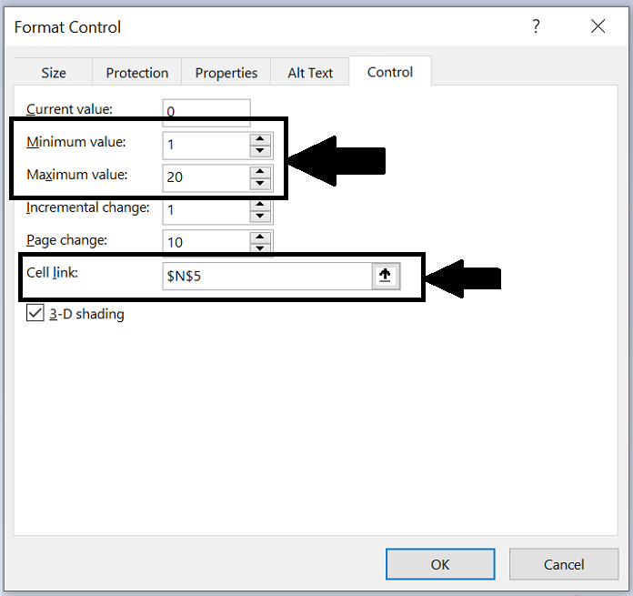
Click on the Control tab in the Format Control dialog box. Then you can specify the Minimum value and Maximum value of your data as you need to, and then click the uparrow button to select the blank cell that will be linked to the scrollbar by clicking the button.

Step 6

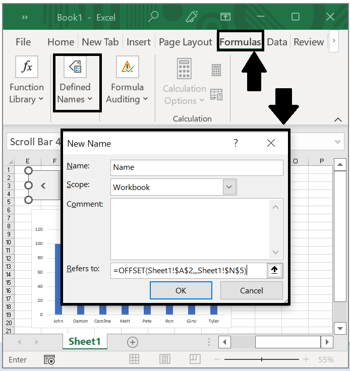
Click on OK to close the dialog box. Select the link cell that you have specified just now to create a range of names you will use after a while. Now next is Click Formulas > Define Name, in the New Name dialog, enter a name for the name range that you want to use. Input the Name then enter this formula =OFFSET(Sheet1!$A$2,,,Sheet1!$N$5) into the refers field ( Sheet1 is the worksheet that you are applied, A2 is the cell that the first data column A without title, N5 is the linked cell that you have specified in Step 5, you can change as you need ).

Step 7

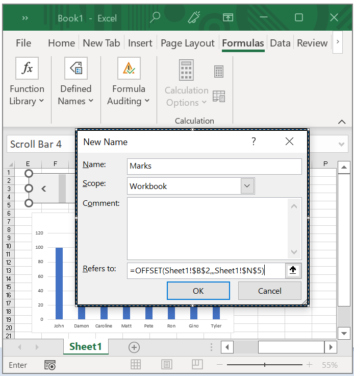
Now click OK and go on clicking Formulas > Define Name to define a name for another range column B as the same as Step 6.

Name: Marks (the defined name for column B )

Refers to: =OFFSET(Sheet1!$B$2,,,Sheet1!$N$5) ( Sheet1 is the worksheet that you are applied, B2 is the cell that the first data in column B without the title, N5 is the linked cell that you have specified in Step 5, you can change as you need).

Step 8

Now click OK to close the dialog and the range names for the chart has been created successfully.

Step 9

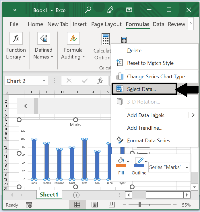
Now you need to link the scrollbar and the chart and right-click the chart area, then choose select data from the context menu.

Step 10

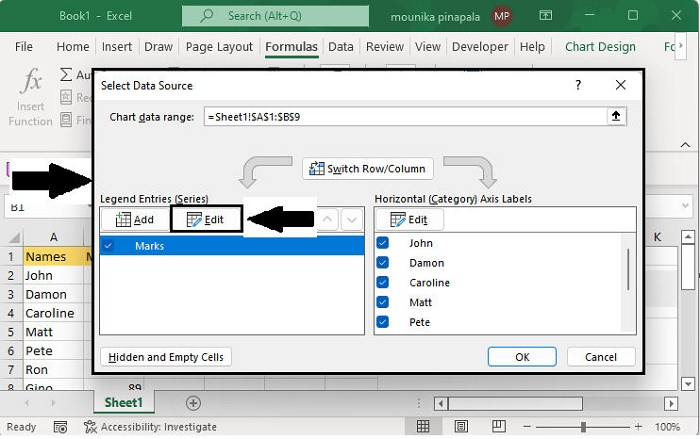
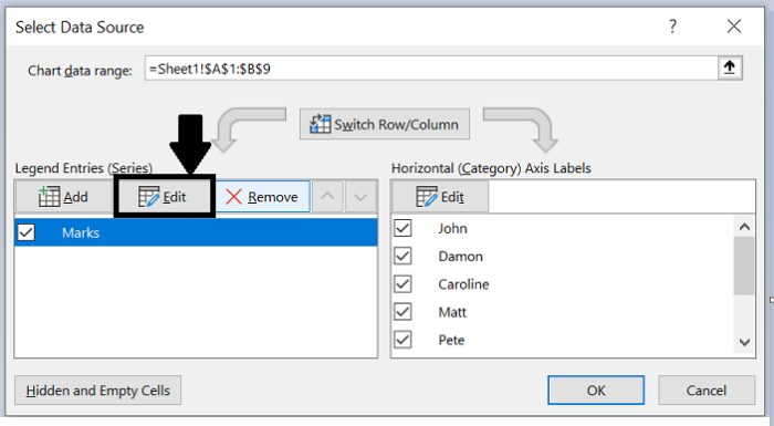
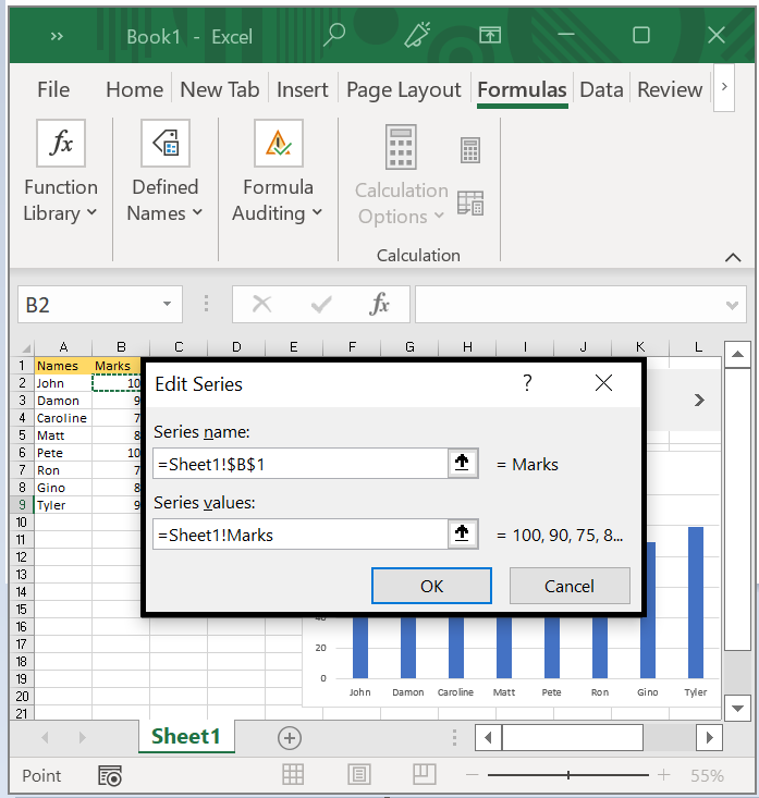
In the select data source dialog, click Marks and click the edit button, in the popped-out edit series dialog, under series name click the up arrow button to select cell B1 and enter this =Sheet1!Marks to the series values field, ( Sheet1 is the worksheet that you are applying and the Marks is the range name that you have created for column B).

Step 11

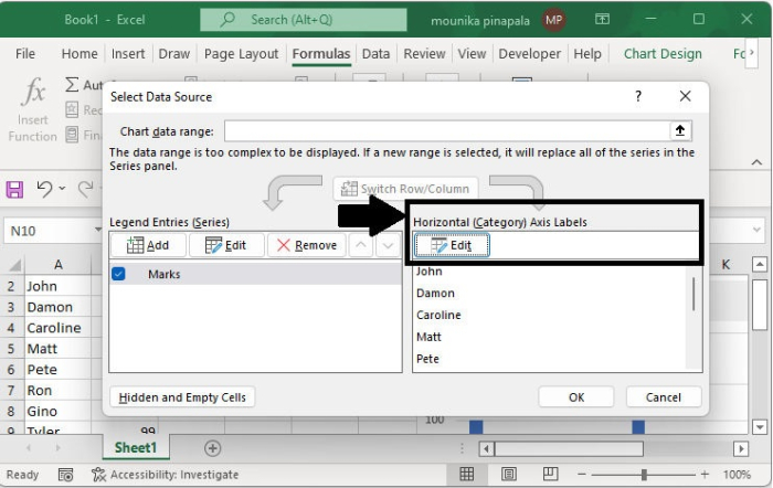
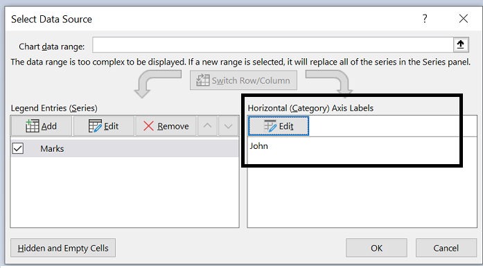
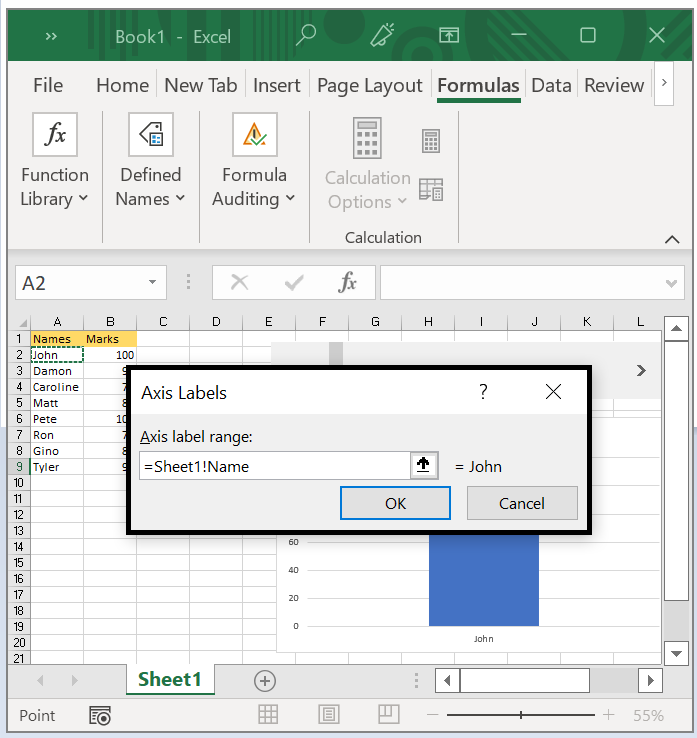
Now click OK to return to the former dialog and in the select data source dialog, click the Edit button under Horizontal axis labels, in the Axis Labels dialog enter =Sheet!Name into the axis label range filed.

Step 12

Click OK > OK to close the dialogs, you have added a scrollbar to the chart. When you drag the scrollbar, the data will be displayed on the chart increasingly.

Step 13

Finally, if you want to combine the scrollbar with the chart, you may select and drag the scrollbar to the chart, then hold down the Ctrl key while selecting the chat and the scrollbar at the same time, and then right-click the scrollbar and select Group > Group from the context menu, and these two objects are combined.

As an example, you can specify the number of data points that should appear on the chart so that you can view the scores of several consecutive data points simultaneously. As a solution to this problem, you just need to specify the number of periods for the chart and change the formulas of the range names that have already been created to solve it.

Insert the scrollbar and then insert the chart. Specify how many periods you wish the data to be displayed for each value in the chart after you insert the scrollbar.