DBMS - Heuristics in Query Processing

---

---

In query processing, we use the concepts of heuristics a lot. Query processing is nothing but the converting user queries into efficient execution plans. Due to the complexity of queries and the vast amounts of data stored in databases, direct query execution can be slow and resource-intensive. And here heuristics come into play.

Heuristics in query processing apply rules or strategies to optimize queries. Using this we can make them more efficient while ensuring correct results. Read this chapter to learn the role of heuristics in query processing and how to apply them in practice.

Heuristics in Query Processing

Heuristics are the guiding principles or rules of thumb. They are used to simplify and improve query execution. They focus on reducing the number of records processed. They minimizing the computation required. Instead of evaluating all possible query execution plans, heuristic based query optimization transforms the query logically using a set of predefined rules.

Heuristics are important due to the following reasons −

• Efficiency − Reduces processing time by avoiding unnecessary operations.
• Simplicity − Gives a straightforward approach compared to cost-based optimization.
• Scalability − Works well for large datasets. This is by minimizing intermediate results.

Query Trees and Query Graphs

Before diving into heuristic rules, it is essential to understand how queries are represented internally in database systems. There are two common representations are query trees and query graphs.

Query Trees

A query tree is a tree. It is a hierarchical structure representing the sequence of operations needed to execute a query. It includes −

• Leaf Nodes − Represent database tables involved in the query.
• Internal Nodes − Represent relational operations such as selection (σ), projection (π), and join (⋈).

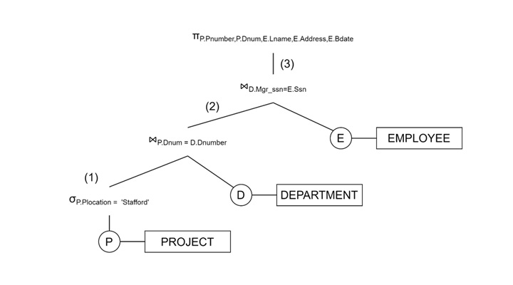
Example − Consider the following query −

Retrieve the project number, controlling department number, and manager's last name, address, and birthdate for every project located in 'Stafford'.

SQL Query:

SELECT P.Pnumber, P.Dnum, E.Lname, E.Address, E.Bdate

FROM PROJECT AS P, DEPARTMENT AS D, EMPLOYEE AS E

WHERE P.Plocation='Stafford' AND P.Dnum=D.Dnumber AND D.Mgr_ssn=E.Ssn;

Query Tree Representation

Leaf Nodes − PROJECT, DEPARTMENT, EMPLOYEE

Operations − Selection (σ), Join (⋈), and Projection (π)

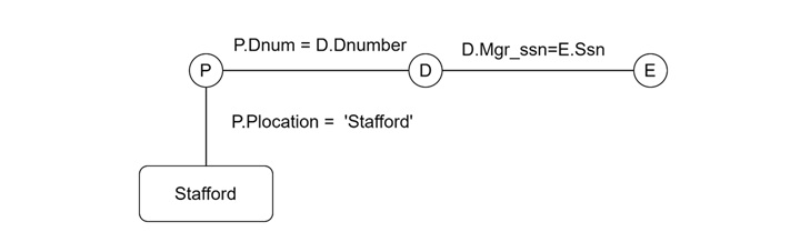
Query Graphs

On the other hand the query graph visually represents relations and operations. Here the relations are displayed as circles, and conditions are represented as edges connecting these circles. Unlike query trees, query graphs do not impose a specific execution order.

Heuristic Rules for Query Optimization

Heuristic query optimization transforms an initial query tree into an optimized execution plan by applying various rules. Let us see the key heuristic rules with examples.

Rule 1: Apply Selections Early

By applying selection operations (σ) as soon as possible it reduces the number of records processed in later stages. This is known as pushing selections down the query tree. For example, consider the following condition −

P.Plocation = 'Stafford'

Apply this selection directly to the PROJECT relation, reducing unnecessary records before the join.

Query Tree Transformation

• Before − PROJECT ⋈ DEPARTMENT ⋈ EMPLOYEE
• After − σ_{P.Plocation = 'Stafford'}(PROJECT) ⋈ DEPARTMENT ⋈ EMPLOYEE

Rule 2: Break Down Selections (Cascading)

If a query has multiple selection conditions, then break them into individual conditions and apply them separately. For example, consider the following condition −

Bdate > '1957-12-31' AND Pname='Aquarius'

Break this into two separate selections −

σBdate > '1957-12-31' (EMPLOYEE)
σPname = 'Aquarius' (PROJECT)

By doing this, each table is filtered independently before combining results.

Rule 3: Perform Joins after Selections

Perform joins only after applying selections. This will minimizes the number of records involved in joins, making the process faster. Consider the following example −

Query − Find employees working on the 'Aquarius' project.

Query Plan −

Apply selection: σPname = 'Aquarius' (PROJECT)

Perform joins −

PROJECT ⋈ P.Pnumber = W.Pno WORKS_ON ⋈ W.Essn = E.Ssn EMPLOYEE 

Rule 4: Apply Projection Early

The projection operations (π) reduce the number of attributes (columns) involved in query execution. Now apply them early to reduce memory usage.

Example: Retrieve only P.Pnumber, P.Dnum, E.Lname, E.Address, and E.Bdate. We are not pulling extra columns through the entire query execution.

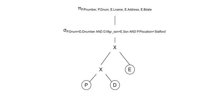
Rule 5: Replace Cartesian Products with Joins

Avoid using Cartesian products unless absolutely necessary. They are resource-intensive and rarely needed in real-world queries. For example,

Instead of −

PROJECT × DEPARTMENT × EMPLOYEE

Use −

PROJECT ⋈ P.Dnum=D.Dnumber DEPARTMENT ⋈ D.Mgr_ssn = E.Ssn EMPLOYEE 

Rule 6: Combine Operations When Possible

Combine operations to minimize intermediate results and reduce storage needs.

Example − If a query asks for employees working on a specific project then retrieve relevant tuples directly instead of generating intermediate tables.

Heuristic Query Transformation Example

Let us see a complete example to see heuristics in action −

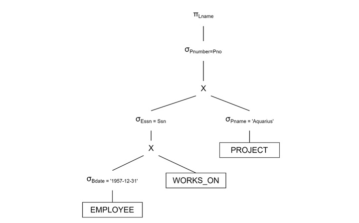
Query − Find the last names of employees born after 1957 who work on a project named 'Aquarius'.

SQL Query −

SELECT E.Lname 

FROM EMPLOYEE AS E, WORKS_ON AS W, PROJECT AS P

WHERE P.Pname = 'Aquarius' AND P.Pnumber = W.Pno AND W.Essn = E.Ssn AND E.Bdate > '1957-12-31';

Initial Query Tree (Unoptimized)

Start with the Cartesian product of EMPLOYEE, WORKS_ON, and PROJECT. Apply selection conditions one by one.

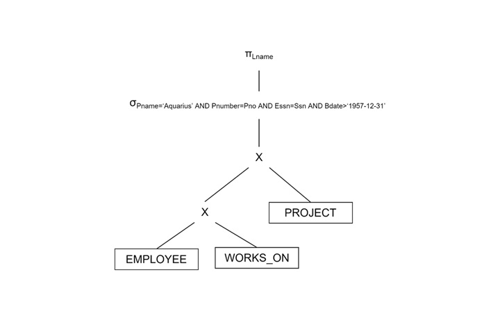
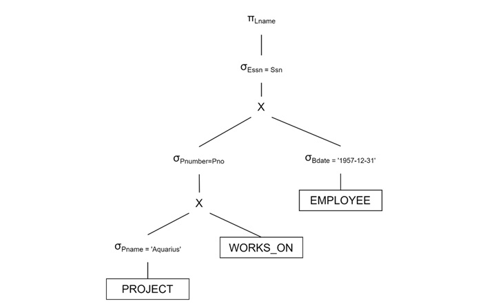
Optimized Query Tree (Using Heuristics)

Apply Selections First:

• σ_Pname = 'Aquarius' (PROJECT) filters relevant projects
• σ_Bdate > '1957-12-31' (EMPLOYEE) filters employees

We can make this optimized as follows −

Perform Joins

• Join PROJECT with WORKS_ON using P.Pnumber = W.Pno.
• Join the result with EMPLOYEE using W.Essn = E.Ssn.

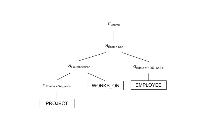
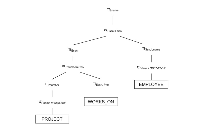
Project the Result

Reduce the join overhead by projecting only required attributes −

Benefits of Heuristic Query Processing

We have understood there are several benefits of using heuristics in query optimization. They are listed below −

• Improved Efficiency − Reduces unnecessary data processing.
• Faster Execution − Shortens execution time by eliminating costly operations.
• Memory Savings − Minimizes intermediate results stored in memory.
• Simpler Query Plans − Creates easy-to-understand query plans.

Challenges and Limitations of Heuristic Query Processing

Apart from the advantages and benefits there are some limitations as well −

• Not Always Optimal − Heuristics are rules of thumb and may not guarantee the best execution plan.
• Complex Queries − Complex queries with multiple joins and conditions may still need cost-based optimization.
• Limited Customization − Heuristic rules are predefined, limiting flexibility in certain scenarios.

Conclusion

In this chapter, we explained how heuristics simplify query processing. This is done by applying logical rules that improve query execution. We understood the importance of query trees and query graphs, and several key heuristic rules such as applying selections early, performing joins efficiently and reducing intermediate results. Through examples and transformations, we explored how databases optimize queries. How to making them faster, scalable, and more efficient for handling large datasets.