DBMS - Multi-level Indexing

Quiz

Data retrieval is the process in database management systems where we need speed and efficiency. We implement the concept of indexing in order to reduce the search time and facilitate faster data retrieval. As databases grow in size, efficient indexing techniques become our primary option to reduce search times. Multi-level indexing is one such indexing technique that is designed to manage large datasets with minimal disk access. Read this chapter to get a good understanding of what multi-level indexing means, what is its structure, and how it works.

What is Multi-level Indexing in DBMS?

In database systems, indexing improves the data retrieval speed by organizing the records in a way that allows faster searches. A single-level index makes a list of key values pointing to corresponding records. This process can be used with a binary search. However, when we are working with massive datasets, a single-level index becomes inefficient due to its size. This is where multi-level indexing is needed for efficiency.

Why Do We Use Multi-level Indexing?

The main reason for using multi-level indexing is to reduce the number of blocks accessed during a search. We know we can apply the binary search where the search space is divided in half at each step. Binary search requires approximately log₂ (b_i) block accesses for an index with b_i blocks. With multi-level indexing, we can improve the search speed by dividing the search space into larger segments. It will reduce the search time exponentially.

For example, instead of cutting the search space in half, we can use multi-level indexing to split it further. This reduces the search space by a factor equal to the fan-out (f₀) value, which denotes the number of entries that can fit into a single block. When the fan-out value is much larger than 2, the search process becomes significantly faster.

Structure of Multi-level Indexing

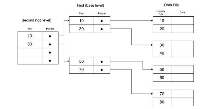
To understand the concept of multi-level indexing, we must know its structures. It is organized into different levels, each representing a progressively smaller index until a manageable size is reached.

The structure consists of −

First Level (Base Level) − This level stores the main index entries. This is also called the base index. It contains unique key values and pointers to corresponding records.
Second Level − This level acts as a primary index for the first level. It stores pointers to the blocks of the first level.
Higher Levels − If the second level becomes too large to fit in a single block, then additional levels are created. It reduces the index size further.

How Does Multi-level Indexing Work?

Each level of the multi-level index reduces the number of entries in the previous level. This is done by the fan-out value (f₀). The process continues until the final level fits into a single block, referred to as the top level.

The number of levels (t) required is calculated as −

$$\mathrm{t \:=\: [log_{f_{0}}(r_{1})]}$$

Where, r₁ is the number of entries in the first level and f₀ is the fan-out value.

From this, it is evident that searching involves retrieving a block from each level and finally accessing the data block. It results in a total of t + 1 block accesses.

Example of Multi-level Indexing

Let us take a detailed example to understand multi-level indexing in action.

The given data is as follows −

Blocking factor (bfri) − 68 entries per block (also called the fan-out, fo).
First-level blocks (b1) − 442 blocks.

Step 1: Calculate the Second Level

We calculate the number of blocks needed at the second level −

$$\mathrm{b_{2} \:=\: \left[\frac{b_{1}}{f_{0}} \right] \:=\: \left[\frac{442}{68} \right] \:=\: 7}$$

The second level has seven blocks.

Step 2: Calculate the Third Level

Similarly, we can calculate the number of blocks needed at the third level −

$$\mathrm{b_{3} \:=\: \left[\frac{b_{2}}{f_{0}} \right] \:=\: \left[\frac{7}{68} \right] \:=\: 1}$$

Since the third level fits into one block, it becomes the top level of the index. This is making the total number of levels t = 3.

Step 3: Record Search Example

After making the index, we must search from it. To search for a record using this multi-level index, we need to access −

One block from each level − Three levels in total.
One data block from the file − The block containing the record.

Total Block Accesses is: T + 1 = 3 + 1 = 4. This is a significant improvement over a single-level index. There are 10 block accesses would have been needed using a binary search.

Types of Multi-level Indexing

Depending on the type of records and access patterns, multi-level indexing can be applied in various forms −

Primary Index − Built on a sorted key field, which makes it sparse (only one index entry per block).
Clustering Index − Built on non-key fields where multiple records share the same value.
Secondary Index − Built on unsorted fields, requiring more maintenance but offering flexibility.

Indexed Sequential Access Method (ISAM)

Indexed Sequential Access Method (ISAM) is a practical implementation of multi-level indexing. ISAM is commonly used in older IBM systems. It uses a two-level index −

Cylinder Index − Points to track-level blocks.
Track Index − Points to specific tracks in the cylinder.

Data insertion is managed using overflow files. This is periodically merged with the main file during reorganization.

Advantages of Multi-level Indexing

Multi-level indexing offers the following benefits −

Faster Searches − Reduces the number of disk accesses.
Scalability − Handles large datasets efficiently.
Supports Different Index Types − Works with primary, clustering, and secondary indexes.
Balanced Access − Ensures near-uniform access times.

One of the major challenges in managing multi-level indexes is during insertions or deletions. It can be complex, as all index levels must be updated. This process becomes problematic when frequent updates occur.

The solution could be dynamic indexing. To address this problem, modern databases use dynamic multi-level indexes such as B − trees and B+ − trees. These structures balance the index by reorganizing the nodes automatically during insertions and deletions.

Conclusion

In this chapter, we explained the concept of multi-level indexing and highlighted its structure and working mechanism. We understood how the search space is reduced through multiple index levels. This technique becomes faster for data retrieval or searching. In addition, we checked a detailed example illustrating how multi-level indexing significantly cuts down on the number of block accesses and makes it much faster than single-level indexing.

Print Page