- Control Systems - Home
- Control Systems - Introduction
- Control Systems - Feedback
- Mathematical Models
- Modelling of Mechanical Systems
- Electrical Analogies of Mechanical Systems
- Control Systems - Block Diagrams
- Block Diagram Algebra
- Block Diagram Reduction
- Signal Flow Graphs
- Mason's Gain Formula
- Time Response Analysis
- Response of the First Order System
- Response of Second Order System
- Time Domain Specifications
- Steady State Errors
- Control Systems - Stability
- Control Systems - Stability Analysis
- Control Systems - Root Locus
- Construction of Root Locus
- Frequency Response Analysis
- Control Systems - Bode Plots
- Construction of Bode Plots
- Control Systems - Polar Plots
- Control Systems - Nyquist Plots
- Control Systems - Compensators
- Control Systems - Controllers
- Control Systems - State Space Model
- State Space Analysis
Control Systems - State Space Model
The state space model of Linear Time-Invariant (LTI) system can be represented as,
$$\dot{X}=AX+BU$$
$$Y=CX+DU$$
The first and the second equations are known as state equation and output equation respectively.
Where,
X and $\dot{X}$ are the state vector and the differential state vector respectively.
U and Y are input vector and output vector respectively.
A is the system matrix.
B and C are the input and the output matrices.
D is the feed-forward matrix.
Basic Concepts of State Space Model
The following basic terminology involved in this chapter.
State
It is a group of variables, which summarizes the history of the system in order to predict the future values (outputs).
State Variable
The number of the state variables required is equal to the number of the storage elements present in the system.
Examples − current flowing through inductor, voltage across capacitor
State Vector
It is a vector, which contains the state variables as elements.
In the earlier chapters, we have discussed two mathematical models of the control systems. Those are the differential equation model and the transfer function model. The state space model can be obtained from any one of these two mathematical models. Let us now discuss these two methods one by one.
State Space Model from Differential Equation
Consider the following series of the RLC circuit. It is having an input voltage, $v_i(t)$ and the current flowing through the circuit is $i(t)$.
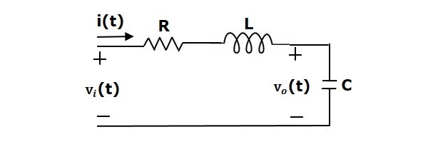
There are two storage elements (inductor and capacitor) in this circuit. So, the number of the state variables is equal to two and these state variables are the current flowing through the inductor, $i(t)$ and the voltage across capacitor, $v_c(t)$.
From the circuit, the output voltage, $v_0(t)$ is equal to the voltage across capacitor, $v_c(t)$.
$$v_0(t)=v_c(t)$$
Apply KVL around the loop.
$$v_i(t)=Ri(t)+L\frac{\text{d}i(t)}{\text{d}t}+v_c(t)$$
$$\Rightarrow \frac{\text{d}i(t)}{\text{d}t}=-\frac{Ri(t)}{L}-\frac{v_c(t)}{L}+\frac{v_i(t)}{L}$$
The voltage across the capacitor is -
$$v_c(t)=\frac{1}{C} \int i(t) dt$$
Differentiate the above equation with respect to time.
$$\frac{\text{d}v_c(t)}{\text{d}t}=\frac{i(t)}{C}$$
State vector, $X=\begin{bmatrix}i(t) \\v_c(t) \end{bmatrix}$
Differential state vector, $\dot{X}=\begin{bmatrix}\frac{\text{d}i(t)}{\text{d}t} \\\frac{\text{d}v_c(t)}{\text{d}t} \end{bmatrix}$
We can arrange the differential equations and output equation into the standard form of state space model as,
$$\dot{X}=\begin{bmatrix}\frac{\text{d}i(t)}{\text{d}t} \\\frac{\text{d}v_c(t)}{\text{d}t} \end{bmatrix}=\begin{bmatrix}-\frac{R}{L} & -\frac{1}{L} \\\frac{1}{C} & 0 \end{bmatrix}\begin{bmatrix}i(t) \\v_c(t) \end{bmatrix}+\begin{bmatrix}\frac{1}{L} \\0 \end{bmatrix}\begin{bmatrix}v_i(t) \end{bmatrix}$$
$$Y=\begin{bmatrix}0 & 1 \end{bmatrix}\begin{bmatrix}i(t) \\v_c(t) \end{bmatrix}$$
Where,
$$A=\begin{bmatrix}-\frac{R}{L} & -\frac{1}{L} \\\frac{1}{C} & 0 \end{bmatrix}, \: B=\begin{bmatrix}\frac{1}{L} \\0 \end{bmatrix}, \: C=\begin{bmatrix}0 & 1 \end{bmatrix} \: and \: D=\begin{bmatrix}0 \end{bmatrix}$$
State Space Model from Transfer Function
Consider the two types of transfer functions based on the type of terms present in the numerator.
- Transfer function having constant term in Numerator.
- Transfer function having polynomial function of s in Numerator.
Transfer function having constant term in Numerator
Consider the following transfer function of a system
$$\frac{Y(s)}{U(s)}=\frac{b_0}{s^n+a_{n-1}s^{n-1}+...+a_1s+a_0}$$
Rearrange, the above equation as
$$(s^n+a_{n-1}s^{n-1}+...+a_0)Y(s)=b_0 U(s)$$
Apply inverse Laplace transform on both sides.
$$\frac{\text{d}^ny(t)}{\text{d}t^n}+a_{n-1}\frac{\text{d}^{n-1}y(t)}{\text{d}t^{n-1}}+...+a_1\frac{\text{d}y(t)}{\text{d}t}+a_0y(t)=b_0 u(t)$$
Let
$$y(t)=x_1$$
$$\frac{\text{d}y(t)}{\text{d}t}=x_2=\dot{x}_1$$
$$\frac{\text{d}^2y(t)}{\text{d}t^2}=x_3=\dot{x}_2$$
$$.$$
$$.$$
$$.$$
$$\frac{\text{d}^{n-1}y(t)}{\text{d}t^{n-1}}=x_n=\dot{x}_{n-1}$$
$$\frac{\text{d}^ny(t)}{\text{d}t^n}=\dot{x}_n$$
and $u(t)=u$
Then,
$$\dot{x}_n+a_{n-1}x_n+...+a_1x_2+a_0x_1=b_0 u$$
From the above equation, we can write the following state equation.
$$\dot{x}_n=-a_0x_1-a_1x_2-...-a_{n-1}x_n+b_0 u$$
The output equation is -
$$y(t)=y=x_1$$
The state space model is -
$\dot{X}=\begin{bmatrix}\dot{x}_1 \\\dot{x}_2 \\\vdots \\\dot{x}_{n-1} \\\dot{x}_n \end{bmatrix}$
$$=\begin{bmatrix}0 & 1 & 0 & \dotso & 0 & 0 \\0 & 0 & 1 & \dotso & 0 & 0 \\\vdots & \vdots & \vdots & \dotso & \vdots & \vdots \\ 0 & 0 & 0 & \dotso & 0 & 1 \\-a_0 & -a_1 & -a_2 & \dotso & -a_{n-2} & -a_{n-1} \end{bmatrix} \begin{bmatrix}x_1 \\x_2 \\\vdots \\x_{n-1} \\x_n \end{bmatrix}+\begin{bmatrix}0 \\0 \\\vdots \\0 \\b_0 \end{bmatrix}\begin{bmatrix}u \end{bmatrix}$$
$$Y=\begin{bmatrix}1 & 0 & \dotso & 0 & 0 \end{bmatrix}\begin{bmatrix}x_1 \\x_2 \\\vdots \\x_{n-1} \\x_n \end{bmatrix}$$
Here, $D=\left [ 0 \right ].$
Example
Find the state space model for the system having transfer function.
$$\frac{Y(s)}{U(s)}=\frac{1}{s^2+s+1}$$
Rearrange, the above equation as,
$$(s^2+s+1)Y(s)=U(s)$$
Apply inverse Laplace transform on both the sides.
$$\frac{\text{d}^2y(t)}{\text{d}t^2}+\frac{\text{d}y(t)}{\text{d}t}+y(t)=u(t)$$
Let
$$y(t)=x_1$$
$$\frac{\text{d}y(t)}{\text{d}t}=x_2=\dot{x}_1$$
and $u(t)=u$
Then, the state equation is
$$\dot{x}_2=-x_1-x_2+u$$
The output equation is
$$y(t)=y=x_1$$
The state space model is
$$\dot{X}=\begin{bmatrix}\dot{x}_1 \\\dot{x}_2 \end{bmatrix}=\begin{bmatrix}0 & 1 \\-1 & -1 \end{bmatrix}\begin{bmatrix}x_1 \\x_2 \end{bmatrix}+\begin{bmatrix}0 \\1 \end{bmatrix}\left [u \right ]$$
$$Y=\begin{bmatrix}1 & 0 \end{bmatrix}\begin{bmatrix}x_1 \\x_2 \end{bmatrix}$$
Transfer function having polynomial function of s in Numerator
Consider the following transfer function of a system
$$\frac{Y(s)}{U(s)}=\frac{b_n s^n+b_{n-1}s^{n-1}+...+b_1s+b_0}{s^n+a_{n-1}s^{n-1}+...+a_1 s+a_0}$$
$$\Rightarrow \frac{Y(s)}{U(s)}=\left( \frac{1}{s^n+a_{n-1}s^{n-1}+...+a_1 s+a_0} \right )(b_n s^n+b_{n-1}s^{n-1}+...+b_1s+b_0)$$
The above equation is in the form of product of transfer functions of two blocks, which are cascaded.
$$\frac{Y(s)}{U(s)}=\left(\frac{V(s)}{U(s)} \right ) \left(\frac{Y(s)}{V(s)} \right )$$
Here,
$$\frac{V(s)}{U(s)}=\frac{1}{s^n+a_{n-1}s^{n-1}+...+a_1 s+a_0}$$
Rearrange, the above equation as
$$(s^n+a_{n-1}s^{n-1}+...+a_0)V(s)=U(s)$$
Apply inverse Laplace transform on both the sides.
$$\frac{\text{d}^nv(t)}{\text{d}t^n}+a_{n-1}\frac{\text{d}^{n-1}v(t)}{\text{d}t^{n-1}}+...+a_1 \frac{\text{d}v(t)}{\text{d}t}+a_0v(t)=u(t)$$
Let
$$v(t)=x_1$$
$$\frac{\text{d}v((t)}{\text{d}t}=x_2=\dot{x}_1$$
$$\frac{\text{d}^2v(t)}{\text{d}t^2}=x_3=\dot{x}_2$$
$$.$$
$$.$$
$$.$$
$$\frac{\text{d}^{n-1}v(t)}{\text{d}t^{n-1}}=x_n=\dot{x}_{n-1}$$
$$\frac{\text{d}^nv(t)}{\text{d}t^n}=\dot{x}_n$$
and $u(t)=u$
Then, the state equation is
$$\dot{x}_n=-a_0x_1-a_1x_2-...-a_{n-1}x_n+u$$
Consider,
$$\frac{Y(s)}{V(s)}=b_ns^n+b_{n-1}s^{n-1}+...+b_1s+b_0$$
Rearrange, the above equation as
$$Y(s)=(b_ns^n+b_{n-1}s^{n-1}+...+b_1s+b_0)V(s)$$
Apply inverse Laplace transform on both the sides.
$$y(t)=b_n\frac{\text{d}^nv(t)}{\text{d}t^n}+b_{n-1}\frac{\text{d}^{n-1}v(t)}{\text{d}t^{n-1}}+...+b_1\frac{\text{d}v(t)}{\text{d}t}+b_0v(t)$$
By substituting the state variables and $y(t)=y$ in the above equation, will get the output equation as,
$$y=b_n\dot{x}_n+b_{n-1}x_n+...+b_1x_2+b_0x_1$$
Substitute, $\dot{x}_n$ value in the above equation.
$$y=b_n(-a_0x_1-a_1x_2-...-a_{n-1}x_n+u)+b_{n-1}x_n+...+b_1x_2+b_0x_1$$
$$y=(b_0-b_na_0)x_1+(b_1-b_na_1)x_2+...+(b_{n-1}-b_na_{n-1})x_n+b_n u$$
The state space model is
$\dot{X}=\begin{bmatrix}\dot{x}_1 \\\dot{x}_2 \\\vdots \\\dot{x}_{n-1} \\\dot{x}_n \end{bmatrix}$
$$=\begin{bmatrix}0 & 1 & 0 & \dotso & 0 & 0 \\0 & 0 & 1 & \dotso & 0 & 0 \\\vdots & \vdots & \vdots & \dotso & \vdots & \vdots \\ 0 & 0 & 0 & \dotso & 0 & 1 \\-a_0 & -a_1 & -a_2 & \dotso & -a_{n-2} & -a_{n-1} \end{bmatrix} \begin{bmatrix}x_1 \\x_2 \\\vdots \\x_{n-1} \\x_n \end{bmatrix}+\begin{bmatrix}0 \\0 \\\vdots \\0 \\b_0 \end{bmatrix}\begin{bmatrix}u \end{bmatrix}$$
$$Y=[b_0-b_na_0 \quad b_1-b_na_1 \quad ... \quad b_{n-2}-b_na_{n-2} \quad b_{n-1}-b_na_{n-1}]\begin{bmatrix}x_1 \\x_2 \\\vdots \\x_{n-1} \\x_n \end{bmatrix}$$
If $b_n = 0$, then,
$$Y=[b_0 \quad b_1 \quad ...\quad b_{n-2} \quad b_{n-1}]\begin{bmatrix}x_1 \\x_2 \\\vdots \\x_{n-1} \\x_n \end{bmatrix}$$
