
- Control Systems - Home
- Control Systems - Introduction
- Control Systems - Feedback
- Mathematical Models
- Modelling of Mechanical Systems
- Electrical Analogies of Mechanical Systems
- Control Systems - Block Diagrams
- Block Diagram Algebra
- Block Diagram Reduction
- Signal Flow Graphs
- Mason's Gain Formula
- Time Response Analysis
- Response of the First Order System
- Response of Second Order System
- Time Domain Specifications
- Steady State Errors
- Control Systems - Stability
- Control Systems - Stability Analysis
- Control Systems - Root Locus
- Construction of Root Locus
- Frequency Response Analysis
- Control Systems - Bode Plots
- Construction of Bode Plots
- Control Systems - Polar Plots
- Control Systems - Nyquist Plots
- Control Systems - Compensators
- Control Systems - Controllers
- Control Systems - State Space Model
- State Space Analysis
Construction of Root Locus
The root locus is a graphical representation in s-domain and it is symmetrical about the real axis. Because the open loop poles and zeros exist in the s-domain having the values either as real or as complex conjugate pairs. In this chapter, let us discuss how to construct (draw) the root locus.
Rules for Construction of Root Locus
Follow these rules for constructing a root locus.
Rule 1 − Locate the open loop poles and zeros in the s plane.
Rule 2 − Find the number of root locus branches.
We know that the root locus branches start at the open loop poles and end at open loop zeros. So, the number of root locus branches N is equal to the number of finite open loop poles P or the number of finite open loop zeros Z, whichever is greater.
Mathematically, we can write the number of root locus branches N as
$N=P$ if $P\geq Z$
$N=Z$ if $P<Z$
Rule 3 − Identify and draw the real axis root locus branches.
If the angle of the open loop transfer function at a point is an odd multiple of 1800, then that point is on the root locus. If odd number of the open loop poles and zeros exist to the left side of a point on the real axis, then that point is on the root locus branch. Therefore, the branch of points which satisfies this condition is the real axis of the root locus branch.
Rule 4 − Find the centroid and the angle of asymptotes.
If $P = Z$, then all the root locus branches start at finite open loop poles and end at finite open loop zeros.
If $P > Z$ , then $Z$ number of root locus branches start at finite open loop poles and end at finite open loop zeros and $P Z$ number of root locus branches start at finite open loop poles and end at infinite open loop zeros.
If $P < Z$ , then P number of root locus branches start at finite open loop poles and end at finite open loop zeros and $Z P$ number of root locus branches start at infinite open loop poles and end at finite open loop zeros.
So, some of the root locus branches approach infinity, when $P \neq Z$. Asymptotes give the direction of these root locus branches. The intersection point of asymptotes on the real axis is known as centroid.
We can calculate the centroid α by using this formula,
$\alpha = \frac{\sum Real\: part\: of\: finite\: open\: loop\: poles\:-\sum Real\: part\: of\: finite\: open\: loop\: zeros}{P-Z}$
The formula for the angle of asymptotes θ is
$$\theta=\frac{(2q+1)180^0}{P-Z}$$
Where,
$$q=0,1,2,....,(P-Z)-1$$
Rule 5 − Find the intersection points of root locus branches with an imaginary axis.
We can calculate the point at which the root locus branch intersects the imaginary axis and the value of K at that point by using the Routh array method and special case (ii).
If all elements of any row of the Routh array are zero, then the root locus branch intersects the imaginary axis and vice-versa.
Identify the row in such a way that if we make the first element as zero, then the elements of the entire row are zero. Find the value of K for this combination.
Substitute this K value in the auxiliary equation. You will get the intersection point of the root locus branch with an imaginary axis.
Rule 6 − Find Break-away and Break-in points.
If there exists a real axis root locus branch between two open loop poles, then there will be a break-away point in between these two open loop poles.
If there exists a real axis root locus branch between two open loop zeros, then there will be a break-in point in between these two open loop zeros.
Note − Break-away and break-in points exist only on the real axis root locus branches.
Follow these steps to find break-away and break-in points.
Write $K$ in terms of $s$ from the characteristic equation $1 + G(s)H(s) = 0$.
Differentiate $K$ with respect to s and make it equal to zero. Substitute these values of $s$ in the above equation.
The values of $s$ for which the $K$ value is positive are the break points.
Rule 7 − Find the angle of departure and the angle of arrival.
The Angle of departure and the angle of arrival can be calculated at complex conjugate open loop poles and complex conjugate open loop zeros respectively.
The formula for the angle of departure $\phi_d$ is
$$\phi_d=180^0-\phi$$
The formula for the angle of arrival $\phi_a$ is
$$\phi_a=180^0+\phi$$
Where,
$$\phi=\sum \phi_P-\sum \phi_Z$$
Example
Let us now draw the root locus of the control system having open loop transfer function, $G(s)H(s)=\frac{K}{s(s+1)(s+5)}$
Step 1 − The given open loop transfer function has three poles at $s = 0, s = 1$ and $s = 5$. It doesnt have any zero. Therefore, the number of root locus branches is equal to the number of poles of the open loop transfer function.
$$N=P=3$$
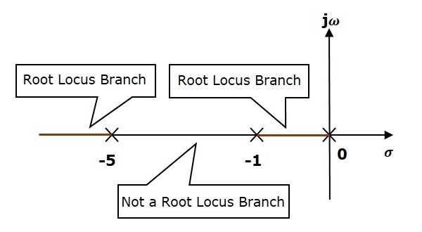
The three poles are located are shown in the above figure. The line segment between $s = 1$ and $s = 0$ is one branch of root locus on real axis. And the other branch of the root locus on the real axis is the line segment to the left of $s = 5$.
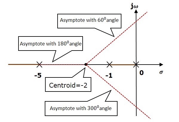
Step 2 − We will get the values of the centroid and the angle of asymptotes by using the given formulae.
Centroid $\alpha = 2$
The angle of asymptotes are $\theta = 60^0,180^0$ and $300^0$.
The centroid and three asymptotes are shown in the following figure.
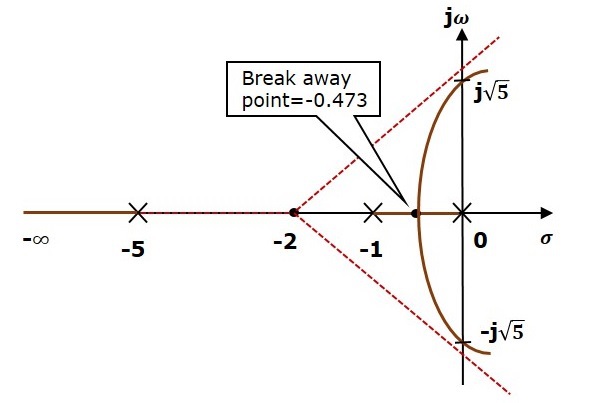
Step 3 − Since two asymptotes have the angles of $60^0$ and $300^0$, two root locus branches intersect the imaginary axis. By using the Routh array method and special case(ii), the root locus branches intersects the imaginary axis at $j\sqrt{5}$ and $j\sqrt{5}$.
There will be one break-away point on the real axis root locus branch between the poles $s = 1$ and $s = 0$. By following the procedure given for the calculation of break-away point, we will get it as $s = 0.473$.
The root locus diagram for the given control system is shown in the following figure.
In this way, you can draw the root locus diagram of any control system and observe the movement of poles of the closed loop transfer function.
From the root locus diagrams, we can know the range of K values for different types of damping.
Effects of Adding Open Loop Poles and Zeros on Root Locus
The root locus can be shifted in s plane by adding the open loop poles and the open loop zeros.
If we include a pole in the open loop transfer function, then some of root locus branches will move towards right half of s plane. Because of this, the damping ratio $\delta$ decreases. Which implies, damped frequency $\omega_d$ increases and the time domain specifications like delay time $t_d$, rise time $t_r$ and peak time $t_p$ decrease. But, it effects the system stability.
If we include a zero in the open loop transfer function, then some of root locus branches will move towards left half of s plane. So, it will increase the control system stability. In this case, the damping ratio $\delta$ increases. Which implies, damped frequency $\omega_d$ decreases and the time domain specifications like delay time $t_d$, rise time $t_r$ and peak time $t_p$ increase.
So, based on the requirement, we can include (add) the open loop poles or zeros to the transfer function.
