
- Control Systems - Home
- Control Systems - Introduction
- Control Systems - Feedback
- Mathematical Models
- Modelling of Mechanical Systems
- Electrical Analogies of Mechanical Systems
- Control Systems - Block Diagrams
- Block Diagram Algebra
- Block Diagram Reduction
- Signal Flow Graphs
- Mason's Gain Formula
- Time Response Analysis
- Response of the First Order System
- Response of Second Order System
- Time Domain Specifications
- Steady State Errors
- Control Systems - Stability
- Control Systems - Stability Analysis
- Control Systems - Root Locus
- Construction of Root Locus
- Frequency Response Analysis
- Control Systems - Bode Plots
- Construction of Bode Plots
- Control Systems - Polar Plots
- Control Systems - Nyquist Plots
- Control Systems - Compensators
- Control Systems - Controllers
- Control Systems - State Space Model
- State Space Analysis
Control Systems - Bode Plots
The Bode plot or the Bode diagram consists of two plots −
- Magnitude plot
- Phase plot
In both the plots, x-axis represents angular frequency (logarithmic scale). Whereas, yaxis represents the magnitude (linear scale) of open loop transfer function in the magnitude plot and the phase angle (linear scale) of the open loop transfer function in the phase plot.
The magnitude of the open loop transfer function in dB is -
$$M=20\: \log|G(j\omega)H(j\omega)|$$
The phase angle of the open loop transfer function in degrees is -
$$\phi=\angle G(j\omega)H(j\omega)$$
Note − The base of logarithm is 10.
Basic of Bode Plots
The following table shows the slope, magnitude and the phase angle values of the terms present in the open loop transfer function. This data is useful while drawing the Bode plots.
| Type of term | G(jω)H(jω) | Slope(dB/dec) | Magnitude (dB) | Phase angle(degrees) |
|---|---|---|---|---|
Constant |
$K$ |
$0$ |
$20 \log K$ |
$0$ |
Zero at origin |
$j\omega$ |
$20$ |
$20 \log \omega$ |
$90$ |
n zeros at origin |
$(j\omega)^n$ |
$20\: n$ |
$20\: n \log \omega$ |
$90\: n$ |
Pole at origin |
$\frac{1}{j\omega}$ |
$-20$ |
$-20 \log \omega$ |
$-90 \: or \: 270$ |
n poles at origin |
$\frac{1}{(j\omega)^n}$ |
$-20\: n$ |
$-20 \: n \log \omega$ |
$-90 \: n \: or \: 270 \: n$ |
Simple zero |
$1+j\omega r$ |
$20$ |
$0\: for\: \omega < \frac{1}{r}$ $20\: \log \omega r\: for \: \omega > \frac{1}{r}$ |
$0 \: for \: \omega < \frac{1}{r}$ $90 \: for \: \omega > \frac{1}{r}$ |
Simple pole |
$\frac{1}{1+j\omega r}$ |
$-20$ |
$0\: for\: \omega < \frac{1}{r}$ $-20\: \log \omega r\: for\: \omega > \frac{1}{r}$ |
$0 \: for \: \omega < \frac{1}{r}$ $-90\: or \: 270 \: for\: \omega > \frac{1}{r}$ |
Second order derivative term |
$\omega_n^2\left ( 1-\frac{\omega^2}{\omega_n^2}+\frac{2j\delta\omega}{\omega_n} \right )$ |
$40$ |
$40\: \log\: \omega_n\: for \: \omega < \omega_n$ $20\: \log\:(2\delta\omega_n^2)\: for \: \omega=\omega_n$ $40 \: \log \: \omega\:for \:\omega > \omega_n$ |
$0 \: for \: \omega < \omega_n$ $90 \: for \: \omega = \omega_n$ $180 \: for \: \omega > \omega_n$ |
Second order integral term |
$\frac{1}{\omega_n^2\left ( 1-\frac{\omega^2}{\omega_n^2}+\frac{2j\delta\omega}{\omega_n} \right )}$ |
$-40$ |
$-40\: \log\: \omega_n\: for \: \omega < \omega_n$ $-20\: \log\:(2\delta\omega_n^2)\: for \: \omega=\omega_n$ $-40 \: \log \: \omega\:for \:\omega > \omega_n$ |
$-0 \: for \: \omega < \omega_n$ $-90 \: for \: \omega = \omega_n$ $-180 \: for \: \omega > \omega_n$ |
Consider the open loop transfer function $G(s)H(s) = K$.
Magnitude $M = 20\: \log K$ dB
Phase angle $\phi = 0$ degrees
If $K = 1$, then magnitude is 0 dB.
If $K > 1$, then magnitude will be positive.
If $K < 1$, then magnitude will be negative.
The following figure shows the corresponding Bode plot.
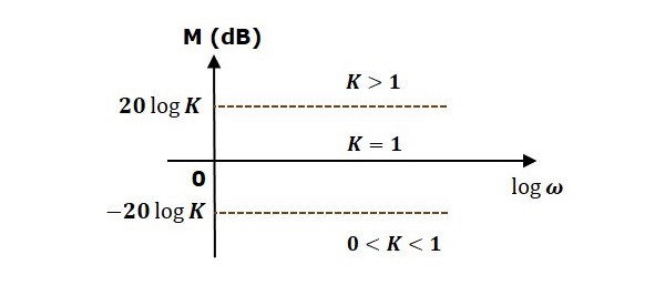
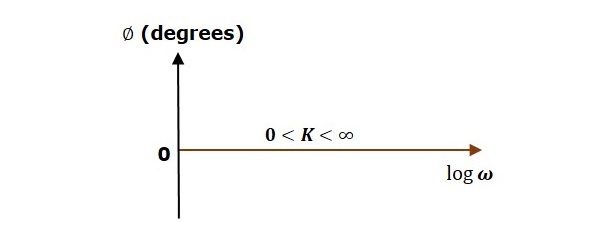
The magnitude plot is a horizontal line, which is independent of frequency. The 0 dB line itself is the magnitude plot when the value of K is one. For the positive values of K, the horizontal line will shift $20 \:\log K$ dB above the 0 dB line. For the negative values of K, the horizontal line will shift $20\: \log K$ dB below the 0 dB line. The Zero degrees line itself is the phase plot for all the positive values of K.
Consider the open loop transfer function $G(s)H(s) = s$.
Magnitude $M = 20 \log \omega$ dB
Phase angle $\phi = 90^0$
At $\omega = 0.1$ rad/sec, the magnitude is -20 dB.
At $\omega = 1$ rad/sec, the magnitude is 0 dB.
At $\omega = 10$ rad/sec, the magnitude is 20 dB.
The following figure shows the corresponding Bode plot.
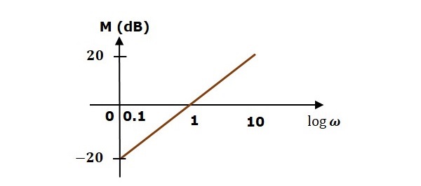
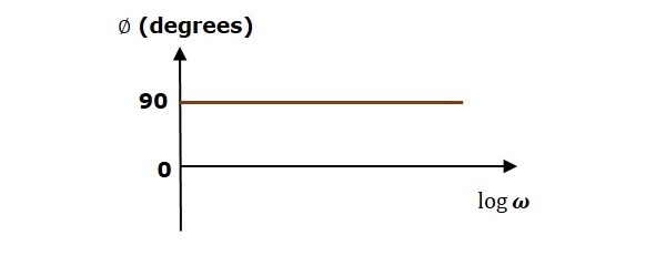
The magnitude plot is a line, which is having a slope of 20 dB/dec. This line started at $\omega = 0.1$ rad/sec having a magnitude of -20 dB and it continues on the same slope. It is touching 0 dB line at $\omega = 1$ rad/sec. In this case, the phase plot is 900 line.
Consider the open loop transfer function $G(s)H(s) = 1 + s\tau$.
Magnitude $M = 20\: log \sqrt{1 + \omega^2\tau^2}$ dB
Phase angle $\phi = \tan^{-1}\omega\tau$ degrees
For $ < \frac{1}{\tau}$ , the magnitude is 0 dB and phase angle is 0 degrees.
For $\omega > \frac{1}{\tau}$ , the magnitude is $20\: \log \omega\tau$ dB and phase angle is 900.
The following figure shows the corresponding Bode plot.
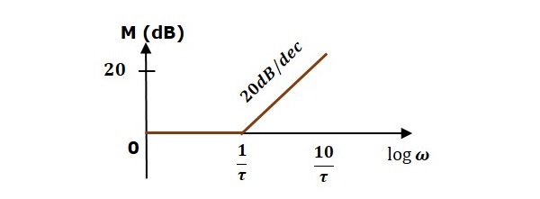
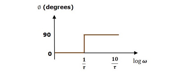
The magnitude plot is having magnitude of 0 dB upto $\omega=\frac{1}{\tau}$ rad/sec. From $\omega = \frac{1}{\tau}$ rad/sec, it is having a slope of 20 dB/dec. In this case, the phase plot is having phase angle of 0 degrees up to $\omega = \frac{1}{\tau}$ rad/sec and from here, it is having phase angle of 900. This Bode plot is called the asymptotic Bode plot.
As the magnitude and the phase plots are represented with straight lines, the Exact Bode plots resemble the asymptotic Bode plots. The only difference is that the Exact Bode plots will have simple curves instead of straight lines.
Similarly, you can draw the Bode plots for other terms of the open loop transfer function which are given in the table.
