
- Control Systems - Home
- Control Systems - Introduction
- Control Systems - Feedback
- Mathematical Models
- Modelling of Mechanical Systems
- Electrical Analogies of Mechanical Systems
- Control Systems - Block Diagrams
- Block Diagram Algebra
- Block Diagram Reduction
- Signal Flow Graphs
- Mason's Gain Formula
- Time Response Analysis
- Response of the First Order System
- Response of Second Order System
- Time Domain Specifications
- Steady State Errors
- Control Systems - Stability
- Control Systems - Stability Analysis
- Control Systems - Root Locus
- Construction of Root Locus
- Frequency Response Analysis
- Control Systems - Bode Plots
- Construction of Bode Plots
- Control Systems - Polar Plots
- Control Systems - Nyquist Plots
- Control Systems - Compensators
- Control Systems - Controllers
- Control Systems - State Space Model
- State Space Analysis
Control Systems - Quick Guide
Control Systems - Introduction
A control system is a system, which provides the desired response by controlling the output. The following figure shows the simple block diagram of a control system.
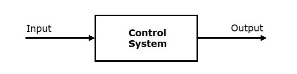
Here, the control system is represented by a single block. Since, the output is controlled by varying input, the control system got this name. We will vary this input with some mechanism. In the next section on open loop and closed loop control systems, we will study in detail about the blocks inside the control system and how to vary this input in order to get the desired response.
Examples − Traffic lights control system, washing machine
Traffic lights control system is an example of control system. Here, a sequence of input signal is applied to this control system and the output is one of the three lights that will be on for some duration of time. During this time, the other two lights will be off. Based on the traffic study at a particular junction, the on and off times of the lights can be determined. Accordingly, the input signal controls the output. So, the traffic lights control system operates on time basis.
Classification of Control Systems
Based on some parameters, we can classify the control systems into the following ways.
Continuous time and Discrete-time Control Systems
Control Systems can be classified as continuous time control systems and discrete time control systems based on the type of the signal used.
In continuous time control systems, all the signals are continuous in time. But, in discrete time control systems, there exists one or more discrete time signals.
SISO and MIMO Control Systems
Control Systems can be classified as SISO control systems and MIMO control systems based on the number of inputs and outputs present.
SISO (Single Input and Single Output) control systems have one input and one output. Whereas, MIMO (Multiple Inputs and Multiple Outputs) control systems have more than one input and more than one output.
Open Loop and Closed Loop Control Systems
Control Systems can be classified as open loop control systems and closed loop control systems based on the feedback path.
In open loop control systems, output is not fed-back to the input. So, the control action is independent of the desired output.
The following figure shows the block diagram of the open loop control system.
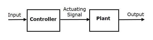
Here, an input is applied to a controller and it produces an actuating signal or controlling signal. This signal is given as an input to a plant or process which is to be controlled. So, the plant produces an output, which is controlled. The traffic lights control system which we discussed earlier is an example of an open loop control system.
In closed loop control systems, output is fed back to the input. So, the control action is dependent on the desired output.
The following figure shows the block diagram of negative feedback closed loop control system.
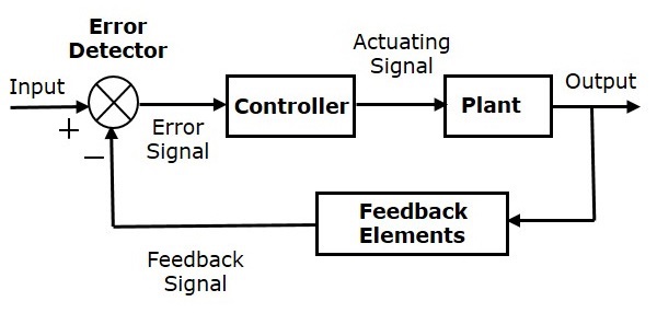
The error detector produces an error signal, which is the difference between the input and the feedback signal. This feedback signal is obtained from the block (feedback elements) by considering the output of the overall system as an input to this block. Instead of the direct input, the error signal is applied as an input to a controller.
So, the controller produces an actuating signal which controls the plant. In this combination, the output of the control system is adjusted automatically till we get the desired response. Hence, the closed loop control systems are also called the automatic control systems. Traffic lights control system having sensor at the input is an example of a closed loop control system.
The differences between the open loop and the closed loop control systems are mentioned in the following table.
| Open Loop Control Systems | Closed Loop Control Systems |
|---|---|
| Control action is independent of the desired output. | Control action is dependent of the desired output. |
| Feedback path is not present. | Feedback path is present. |
| These are also called as non-feedback control systems. | These are also called as feedback control systems. |
| Easy to design. | Difficult to design. |
| These are economical. | These are costlier. |
| Inaccurate. | Accurate. |
Control Systems - Feedback
If either the output or some part of the output is returned to the input side and utilized as part of the system input, then it is known as feedback. Feedback plays an important role in order to improve the performance of the control systems. In this chapter, let us discuss the types of feedback & effects of feedback.
Types of Feedback
There are two types of feedback −
- Positive feedback
- Negative feedback
Positive Feedback
The positive feedback adds the reference input, $R(s)$ and feedback output. The following figure shows the block diagram of positive feedback control system.
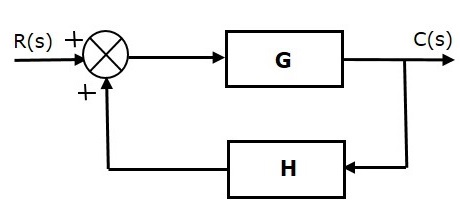
The concept of transfer function will be discussed in later chapters. For the time being, consider the transfer function of positive feedback control system is,
$T=\frac{G}{1-GH}$ (Equation 1)
Where,
T is the transfer function or overall gain of positive feedback control system.
G is the open loop gain, which is function of frequency.
H is the gain of feedback path, which is function of frequency.
Negative Feedback
Negative feedback reduces the error between the reference input, $R(s)$ and system output. The following figure shows the block diagram of the negative feedback control system.
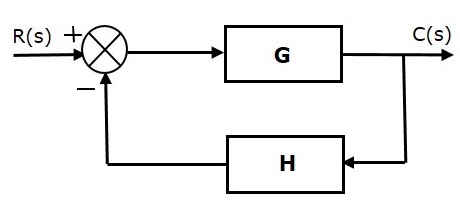
Transfer function of negative feedback control system is,
$T=\frac{G}{1+GH}$ (Equation 2)
Where,
T is the transfer function or overall gain of negative feedback control system.
G is the open loop gain, which is function of frequency.
H is the gain of feedback path, which is function of frequency.
The derivation of the above transfer function is present in later chapters.
Effects of Feedback
Let us now understand the effects of feedback.
Effect of Feedback on Overall Gain
From Equation 2, we can say that the overall gain of negative feedback closed loop control system is the ratio of 'G' and (1+GH). So, the overall gain may increase or decrease depending on the value of (1+GH).
If the value of (1+GH) is less than 1, then the overall gain increases. In this case, 'GH' value is negative because the gain of the feedback path is negative.
If the value of (1+GH) is greater than 1, then the overall gain decreases. In this case, 'GH' value is positive because the gain of the feedback path is positive.
In general, 'G' and 'H' are functions of frequency. So, the feedback will increase the overall gain of the system in one frequency range and decrease in the other frequency range.
Effect of Feedback on Sensitivity
Sensitivity of the overall gain of negative feedback closed loop control system (T) to the variation in open loop gain (G) is defined as
$S_{G}^{T} = \frac{\frac{\partial T}{T}}{\frac{\partial G}{G}}=\frac{Percentage\: change \: in \:T}{Percentage\: change \: in \:G}$ (Equation 3)
Where, ∂T is the incremental change in T due to incremental change in G.
We can rewrite Equation 3 as
$S_{G}^{T}=\frac{\partial T}{\partial G}\frac{G}{T}$ (Equation 4)
Do partial differentiation with respect to G on both sides of Equation 2.
$\frac{\partial T}{\partial G}=\frac{\partial}{\partial G}\left (\frac{G}{1+GH} \right )=\frac{(1+GH).1-G(H)}{(1+GH)^2}=\frac{1}{(1+GH)^2}$ (Equation 5)
From Equation 2, you will get
$\frac{G}{T}=1+GH$ (Equation 6)
Substitute Equation 5 and Equation 6 in Equation 4.
$$S_{G}^{T}=\frac{1}{(1+GH)^2}(1+GH)=\frac{1}{1+GH}$$
So, we got the sensitivity of the overall gain of closed loop control system as the reciprocal of (1+GH). So, Sensitivity may increase or decrease depending on the value of (1+GH).
If the value of (1+GH) is less than 1, then sensitivity increases. In this case, 'GH' value is negative because the gain of feedback path is negative.
If the value of (1+GH) is greater than 1, then sensitivity decreases. In this case, 'GH' value is positive because the gain of feedback path is positive.
In general, 'G' and 'H' are functions of frequency. So, feedback will increase the sensitivity of the system gain in one frequency range and decrease in the other frequency range. Therefore, we have to choose the values of 'GH' in such a way that the system is insensitive or less sensitive to parameter variations.
Effect of Feedback on Stability
A system is said to be stable, if its output is under control. Otherwise, it is said to be unstable.
In Equation 2, if the denominator value is zero (i.e., GH = -1), then the output of the control system will be infinite. So, the control system becomes unstable.
Therefore, we have to properly choose the feedback in order to make the control system stable.
Effect of Feedback on Noise
To know the effect of feedback on noise, let us compare the transfer function relations with and without feedback due to noise signal alone.
Consider an open loop control system with noise signal as shown below.
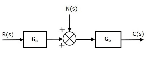
The open loop transfer function due to noise signal alone is
$\frac{C(s)}{N(s)}=G_b$ (Equation 7)
It is obtained by making the other input $R(s)$ equal to zero.
Consider a closed loop control system with noise signal as shown below.
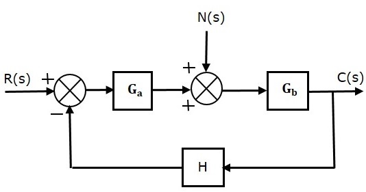
The closed loop transfer function due to noise signal alone is
$\frac{C(s)}{N(s)}=\frac{G_b}{1+G_aG_bH}$ (Equation 8)
It is obtained by making the other input $R(s)$ equal to zero.
Compare Equation 7 and Equation 8,
In the closed loop control system, the gain due to noise signal is decreased by a factor of $(1+G_a G_b H)$ provided that the term $(1+G_a G_b H)$ is greater than one.
Control Systems - Mathematical Models
The control systems can be represented with a set of mathematical equations known as mathematical model. These models are useful for analysis and design of control systems. Analysis of control system means finding the output when we know the input and mathematical model. Design of control system means finding the mathematical model when we know the input and the output.
The following mathematical models are mostly used.
- Differential equation model
- Transfer function model
- State space model
Let us discuss the first two models in this chapter.
Differential Equation Model
Differential equation model is a time domain mathematical model of control systems. Follow these steps for differential equation model.
Apply basic laws to the given control system.
Get the differential equation in terms of input and output by eliminating the intermediate variable(s).
Example
Consider the following electrical system as shown in the following figure. This circuit consists of resistor, inductor and capacitor. All these electrical elements are connected in series. The input voltage applied to this circuit is $v_i$ and the voltage across the capacitor is the output voltage $v_o$.
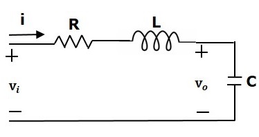
Mesh equation for this circuit is
$$v_i=Ri+L\frac{\text{d}i}{\text{d}t}+v_o$$
Substitute, the current passing through capacitor $i=c\frac{\text{d}v_o}{\text{d}t}$ in the above equation.
$$\Rightarrow\:v_i=RC\frac{\text{d}v_o}{\text{d}t}+LC\frac{\text{d}^2v_o}{\text{d}t^2}+v_o$$
$$\Rightarrow\frac{\text{d}^2v_o}{\text{d}t^2}+\left ( \frac{R}{L} \right )\frac{\text{d}v_o}{\text{d}t}+\left ( \frac{1}{LC} \right )v_o=\left ( \frac{1}{LC} \right )v_i$$
The above equation is a second order differential equation.
Transfer Function Model
Transfer function model is an s-domain mathematical model of control systems. The Transfer function of a Linear Time Invariant (LTI) system is defined as the ratio of Laplace transform of output and Laplace transform of input by assuming all the initial conditions are zero.
If $x(t)$ and $y(t)$ are the input and output of an LTI system, then the corresponding Laplace transforms are $X(s)$ and $Y(s)$.
Therefore, the transfer function of LTI system is equal to the ratio of $Y(s)$ and $X(s)$.
$$i.e.,\: Transfer\: Function =\frac{Y(s)}{X(s)}$$
The transfer function model of an LTI system is shown in the following figure.
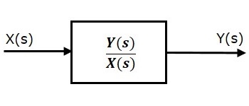
Here, we represented an LTI system with a block having transfer function inside it. And this block has an input $X(s)$ & output $Y(s)$.
Example
Previously, we got the differential equation of an electrical system as
$$\frac{\text{d}^2v_o}{\text{d}t^2}+\left ( \frac{R}{L} \right )\frac{\text{d}v_o}{\text{d}t}+\left ( \frac{1}{LC} \right )v_o=\left ( \frac{1}{LC} \right )v_i$$
Apply Laplace transform on both sides.
$$s^2V_o(s)+\left ( \frac{sR}{L} \right )V_o(s)+\left ( \frac{1}{LC} \right )V_o(s)=\left ( \frac{1}{LC} \right )V_i(s)$$
$$\Rightarrow \left \{ s^2+\left ( \frac{R}{L} \right )s+\frac{1}{LC} \right \}V_o(s)=\left ( \frac{1}{LC} \right )V_i(s)$$
$$\Rightarrow \frac{V_o(s)}{V_i(s)}=\frac{\frac{1}{LC}}{s^2+\left ( \frac{R}{L} \right )s+\frac{1}{LC}}$$
Where,
$v_i(s)$ is the Laplace transform of the input voltage $v_i$
$v_o(s)$ is the Laplace transform of the output voltage $v_o$
The above equation is a transfer function of the second order electrical system. The transfer function model of this system is shown below.
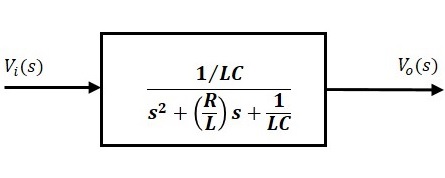
Here, we show a second order electrical system with a block having the transfer function inside it. And this block has an input $V_i(s)$ & an output $V_o(s)$.
Modelling of Mechanical Systems
In this chapter, let us discuss the differential equation modeling of mechanical systems. There are two types of mechanical systems based on the type of motion.
- Translational mechanical systems
- Rotational mechanical systems
Modeling of Translational Mechanical Systems
Translational mechanical systems move along a straight line. These systems mainly consist of three basic elements. Those are mass, spring and dashpot or damper.
If a force is applied to a translational mechanical system, then it is opposed by opposing forces due to mass, elasticity and friction of the system. Since the applied force and the opposing forces are in opposite directions, the algebraic sum of the forces acting on the system is zero. Let us now see the force opposed by these three elements individually.
Mass
Mass is the property of a body, which stores kinetic energy. If a force is applied on a body having mass M, then it is opposed by an opposing force due to mass. This opposing force is proportional to the acceleration of the body. Assume elasticity and friction are negligible.
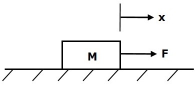
$$F_m\propto\: a$$
$$\Rightarrow F_m=Ma=M\frac{\text{d}^2x}{\text{d}t^2}$$
$$F=F_m=M\frac{\text{d}^2x}{\text{d}t^2}$$
Where,
F is the applied force
Fm is the opposing force due to mass
M is mass
a is acceleration
x is displacement
Spring
Spring is an element, which stores potential energy. If a force is applied on spring K, then it is opposed by an opposing force due to elasticity of spring. This opposing force is proportional to the displacement of the spring. Assume mass and friction are negligible.
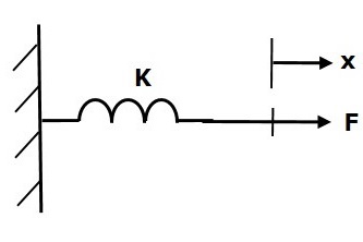
$$F\propto\: x$$
$$\Rightarrow F_k=Kx$$
$$F=F_k=Kx$$
Where,
F is the applied force
Fk is the opposing force due to elasticity of spring
K is spring constant
x is displacement
Dashpot
If a force is applied on dashpot B, then it is opposed by an opposing force due to friction of the dashpot. This opposing force is proportional to the velocity of the body. Assume mass and elasticity are negligible.
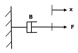
$$F_b\propto\: \nu$$
$$\Rightarrow F_b=B\nu=B\frac{\text{d}x}{\text{d}t}$$
$$F=F_b=B\frac{\text{d}x}{\text{d}t}$$
Where,
Fb is the opposing force due to friction of dashpot
B is the frictional coefficient
v is velocity
x is displacement
Modeling of Rotational Mechanical Systems
Rotational mechanical systems move about a fixed axis. These systems mainly consist of three basic elements. Those are moment of inertia, torsional spring and dashpot.
If a torque is applied to a rotational mechanical system, then it is opposed by opposing torques due to moment of inertia, elasticity and friction of the system. Since the applied torque and the opposing torques are in opposite directions, the algebraic sum of torques acting on the system is zero. Let us now see the torque opposed by these three elements individually.
Moment of Inertia
In translational mechanical system, mass stores kinetic energy. Similarly, in rotational mechanical system, moment of inertia stores kinetic energy.
If a torque is applied on a body having moment of inertia J, then it is opposed by an opposing torque due to the moment of inertia. This opposing torque is proportional to angular acceleration of the body. Assume elasticity and friction are negligible.
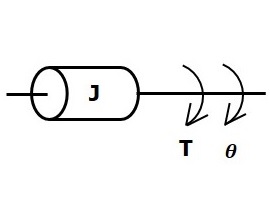
$$T_j\propto\: \alpha$$
$$\Rightarrow T_j=J\alpha=J\frac{\text{d}^2\theta}{\text{d}t^2}$$
$$T=T_j=J\frac{\text{d}^2\theta}{\text{d}t^2}$$
Where,
T is the applied torque
Tj is the opposing torque due to moment of inertia
J is moment of inertia
α is angular acceleration
θ is angular displacement
Torsional Spring
In translational mechanical system, spring stores potential energy. Similarly, in rotational mechanical system, torsional spring stores potential energy.
If a torque is applied on torsional spring K, then it is opposed by an opposing torque due to the elasticity of torsional spring. This opposing torque is proportional to the angular displacement of the torsional spring. Assume that the moment of inertia and friction are negligible.
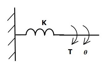
$$T_k\propto\: \theta$$
$$\Rightarrow T_k=K\theta$$
$$T=T_k=K\theta$$
Where,
T is the applied torque
Tk is the opposing torque due to elasticity of torsional spring
K is the torsional spring constant
θ is angular displacement
Dashpot
If a torque is applied on dashpot B, then it is opposed by an opposing torque due to the rotational friction of the dashpot. This opposing torque is proportional to the angular velocity of the body. Assume the moment of inertia and elasticity are negligible.
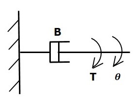
$$T_b\propto\: \omega$$
$$\Rightarrow T_b=B\omega=B\frac{\text{d}\theta}{\text{d}t}$$
$$T=T_b=B\frac{\text{d}\theta}{\text{d}t}$$
Where,
Tb is the opposing torque due to the rotational friction of the dashpot
B is the rotational friction coefficient
ω is the angular velocity
θ is the angular displacement
Electrical Analogies of Mechanical Systems
Two systems are said to be analogous to each other if the following two conditions are satisfied.
- The two systems are physically different
- Differential equation modelling of these two systems are same
Electrical systems and mechanical systems are two physically different systems. There are two types of electrical analogies of translational mechanical systems. Those are force voltage analogy and force current analogy.
Force Voltage Analogy
In force voltage analogy, the mathematical equations of translational mechanical system are compared with mesh equations of the electrical system.
Consider the following translational mechanical system as shown in the following figure.
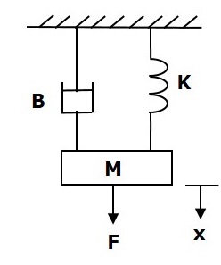
The force balanced equation for this system is
$$F=F_m+F_b+F_k$$
$\Rightarrow F=M\frac{\text{d}^2x}{\text{d}t^2}+B\frac{\text{d}x}{\text{d}t}+Kx$ (Equation 1)
Consider the following electrical system as shown in the following figure. This circuit consists of a resistor, an inductor and a capacitor. All these electrical elements are connected in a series. The input voltage applied to this circuit is $V$ volts and the current flowing through the circuit is $i$ Amps.
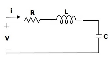
Mesh equation for this circuit is
$V=Ri+L\frac{\text{d}i}{\text{d}t}+\frac{1}{c}\int idt$ (Equation 2)
Substitute, $i=\frac{\text{d}q}{\text{d}t}$ in Equation 2.
$$V=R\frac{\text{d}q}{\text{d}t}+L\frac{\text{d}^2q}{\text{d}t^2}+\frac{q}{C}$$
$\Rightarrow V=L\frac{\text{d}^2q}{\text{d}t^2}+R\frac{\text{d}q}{\text{d}t}+\left ( \frac{1}{c} \right )q$ (Equation 3)
By comparing Equation 1 and Equation 3, we will get the analogous quantities of the translational mechanical system and electrical system. The following table shows these analogous quantities.
| Translational Mechanical System | Electrical System |
|---|---|
| Force(F) | Voltage(V) |
| Mass(M) | Inductance(L) |
| Frictional Coefficient(B) | Resistance(R) |
| Spring Constant(K) | Reciprocal of Capacitance $(\frac{1}{c})$ |
| Displacement(x) | Charge(q) |
| Velocity(v) | Current(i) |
Similarly, there is torque voltage analogy for rotational mechanical systems. Let us now discuss about this analogy.
Torque Voltage Analogy
In this analogy, the mathematical equations of rotational mechanical system are compared with mesh equations of the electrical system.
Rotational mechanical system is shown in the following figure.
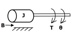
The torque balanced equation is
$$T=T_j+T_b+T_k$$
$\Rightarrow T=J\frac{\text{d}^2\theta}{\text{d}t^2}+B\frac{\text{d}\theta}{\text{d}t}+k\theta$ (Equation 4)
By comparing Equation 4 and Equation 3, we will get the analogous quantities of rotational mechanical system and electrical system. The following table shows these analogous quantities.
| Rotational Mechanical System | Electrical System |
|---|---|
| Torque(T) | Voltage(V) |
| Moment of Inertia(J) | Inductance(L) |
| Rotational friction coefficient(B) | Resistance(R) |
| Torsional spring constant(K) | Reciprocal of Capacitance $(\frac{1}{c})$ |
| Angular Displacement(θ) | Charge(q) |
| Angular Velocity(ω) | Current(i) |
Force Current Analogy
In force current analogy, the mathematical equations of the translational mechanical system are compared with the nodal equations of the electrical system.
Consider the following electrical system as shown in the following figure. This circuit consists of current source, resistor, inductor and capacitor. All these electrical elements are connected in parallel.
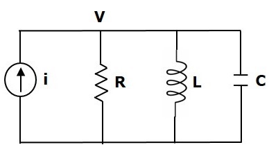
The nodal equation is
$i=\frac{V}{R}+\frac{1}{L}\int Vdt+C\frac{\text{d}V}{\text{d}t}$ (Equation 5)
Substitute, $V=\frac{\text{d}\Psi}{\text{d}t}$ in Equation 5.
$$i=\frac{1}{R}\frac{\text{d}\Psi}{\text{d}t}+\left ( \frac{1}{L} \right )\Psi+C\frac{\text{d}^2\Psi}{\text{d}t^2}$$
$\Rightarrow i=C\frac{\text{d}^2\Psi}{\text{d}t^2}+\left ( \frac{1}{R} \right )\frac{\text{d}\Psi}{\text{d}t}+\left ( \frac{1}{L} \right )\Psi$ (Equation 6)
By comparing Equation 1 and Equation 6, we will get the analogous quantities of the translational mechanical system and electrical system. The following table shows these analogous quantities.
| Translational Mechanical System | Electrical System |
|---|---|
| Force(F) | Current(i) |
| Mass(M) | Capacitance(C) |
| Frictional coefficient(B) | Reciprocal of Resistance$(\frac{1}{R})$ |
| Spring constant(K) | Reciprocal of Inductance$(\frac{1}{L})$ |
| Displacement(x) | Magnetic Flux(ψ) |
| Velocity(v) | Voltage(V) |
Similarly, there is a torque current analogy for rotational mechanical systems. Let us now discuss this analogy.
Torque Current Analogy
In this analogy, the mathematical equations of the rotational mechanical system are compared with the nodal mesh equations of the electrical system.
By comparing Equation 4 and Equation 6, we will get the analogous quantities of rotational mechanical system and electrical system. The following table shows these analogous quantities.
| Rotational Mechanical System | Electrical System |
|---|---|
| Torque(T) | Current(i) |
| Moment of inertia(J) | Capacitance(C) |
| Rotational friction coefficient(B) | Reciprocal of Resistance$(\frac{1}{R})$ |
| Torsional spring constant(K) | Reciprocal of Inductance$(\frac{1}{L})$ |
| Angular displacement(θ) | Magnetic flux(ψ) |
| Angular velocity(ω) | Voltage(V) |
In this chapter, we discussed the electrical analogies of the mechanical systems. These analogies are helpful to study and analyze the non-electrical system like mechanical system from analogous electrical system.
Control Systems - Block Diagrams
Block diagrams consist of a single block or a combination of blocks. These are used to represent the control systems in pictorial form.
Basic Elements of Block Diagram
The basic elements of a block diagram are a block, the summing point and the take-off point. Let us consider the block diagram of a closed loop control system as shown in the following figure to identify these elements.
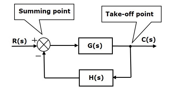
The above block diagram consists of two blocks having transfer functions G(s) and H(s). It is also having one summing point and one take-off point. Arrows indicate the direction of the flow of signals. Let us now discuss these elements one by one.
Block
The transfer function of a component is represented by a block. Block has single input and single output.
The following figure shows a block having input X(s), output Y(s) and the transfer function G(s).

Transfer Function,$G(s)=\frac{Y(s)}{X(s)}$
$$\Rightarrow Y(s)=G(s)X(s)$$
Output of the block is obtained by multiplying transfer function of the block with input.
Summing Point
The summing point is represented with a circle having cross (X) inside it. It has two or more inputs and single output. It produces the algebraic sum of the inputs. It also performs the summation or subtraction or combination of summation and subtraction of the inputs based on the polarity of the inputs. Let us see these three operations one by one.
The following figure shows the summing point with two inputs (A, B) and one output (Y). Here, the inputs A and B have a positive sign. So, the summing point produces the output, Y as sum of A and B.
i.e.,Y = A + B.

The following figure shows the summing point with two inputs (A, B) and one output (Y). Here, the inputs A and B are having opposite signs, i.e., A is having positive sign and B is having negative sign. So, the summing point produces the output Y as the difference of A and B.
Y = A + (-B) = A - B.

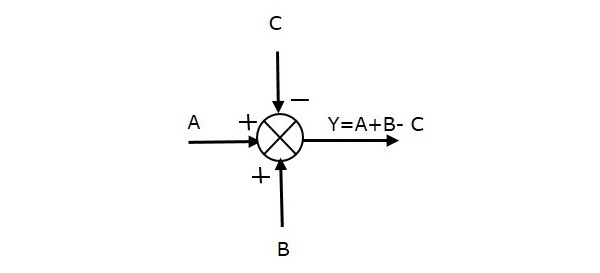
The following figure shows the summing point with three inputs (A, B, C) and one output (Y). Here, the inputs A and B are having positive signs and C is having a negative sign. So, the summing point produces the output Y as
Y = A + B + (C) = A + B C.
Take-off Point
The take-off point is a point from which the same input signal can be passed through more than one branch. That means with the help of take-off point, we can apply the same input to one or more blocks, summing points.
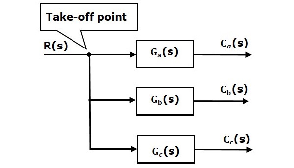
In the following figure, the take-off point is used to connect the same input, R(s) to two more blocks.
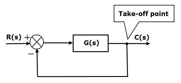
In the following figure, the take-off point is used to connect the output C(s), as one of the inputs to the summing point.
Block Diagram Representation of Electrical Systems
In this section, let us represent an electrical system with a block diagram. Electrical systems contain mainly three basic elements resistor, inductor and capacitor.
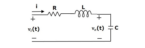
Consider a series of RLC circuit as shown in the following figure. Where, Vi(t) and Vo(t) are the input and output voltages. Let i(t) be the current passing through the circuit. This circuit is in time domain.
By applying the Laplace transform to this circuit, will get the circuit in s-domain. The circuit is as shown in the following figure.
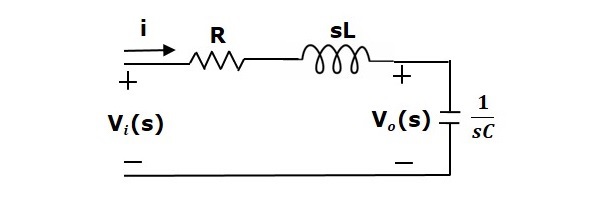
From the above circuit, we can write
$$I(s)=\frac{V_i(s)-V_o(s)}{R+sL}$$
$\Rightarrow I(s)=\left \{ \frac{1}{R+sL} \right \}\left \{ V_i(s)-V_o(s) \right \}$ (Equation 1)
$V_o(s)=\left ( \frac{1}{sC} \right )I(s)$ (Equation 2)
Let us now draw the block diagrams for these two equations individually. And then combine those block diagrams properly in order to get the overall block diagram of series of RLC Circuit (s-domain).
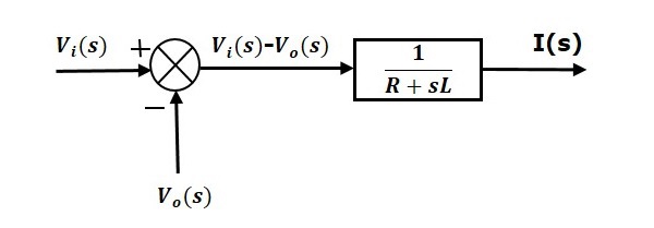
Equation 1 can be implemented with a block having the transfer function, $\frac{1}{R+sL}$. The input and output of this block are $\left \{ V_i(s)-V_o(s) \right \}$ and $I(s)$. We require a summing point to get $\left \{ V_i(s)-V_o(s) \right \}$. The block diagram of Equation 1 is shown in the following figure.
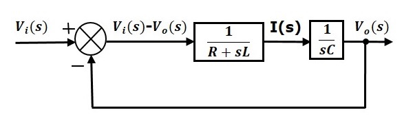
Equation 2 can be implemented with a block having transfer function, $\frac{1}{sC}$. The input and output of this block are $I(s)$ and $V_o(s)$. The block diagram of Equation 2 is shown in the following figure.

The overall block diagram of the series of RLC Circuit (s-domain) is shown in the following figure.
Similarly, you can draw the block diagram of any electrical circuit or system just by following this simple procedure.
Convert the time domain electrical circuit into an s-domain electrical circuit by applying Laplace transform.
Write down the equations for the current passing through all series branch elements and voltage across all shunt branches.
Draw the block diagrams for all the above equations individually.
Combine all these block diagrams properly in order to get the overall block diagram of the electrical circuit (s-domain).
Control Systems - Block Diagram Algebra
Block diagram algebra is nothing but the algebra involved with the basic elements of the block diagram. This algebra deals with the pictorial representation of algebraic equations.
Basic Connections for Blocks
There are three basic types of connections between two blocks.
Series Connection
Series connection is also called cascade connection. In the following figure, two blocks having transfer functions $G_1(s)$ and $G_2(s)$ are connected in series.
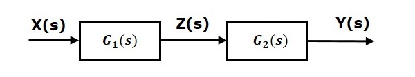
For this combination, we will get the output $Y(s)$ as
$$Y(s)=G_2(s)Z(s)$$
Where, $Z(s)=G_1(s)X(s)$
$$\Rightarrow Y(s)=G_2(s)[G_1(s)X(s)]=G_1(s)G_2(s)X(s)$$
$$\Rightarrow Y(s)=\lbrace G_1(s)G_2(s)\rbrace X(s)$$
Compare this equation with the standard form of the output equation, $Y(s)=G(s)X(s)$. Where, $G(s) = G_1(s)G_2(s)$.
That means we can represent the series connection of two blocks with a single block. The transfer function of this single block is the product of the transfer functions of those two blocks. The equivalent block diagram is shown below.

Similarly, you can represent series connection of n blocks with a single block. The transfer function of this single block is the product of the transfer functions of all those n blocks.
Parallel Connection
The blocks which are connected in parallel will have the same input. In the following figure, two blocks having transfer functions $G_1(s)$ and $G_2(s)$ are connected in parallel. The outputs of these two blocks are connected to the summing point.
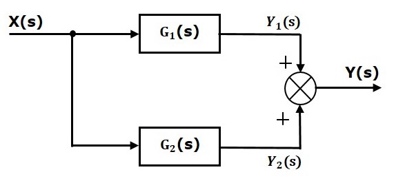
For this combination, we will get the output $Y(s)$ as
$$Y(s)=Y_1(s)+Y_2(s)$$
Where, $Y_1(s)=G_1(s)X(s)$ and $Y_2(s)=G_2(s)X(s)$
$$\Rightarrow Y(s)=G_1(s)X(s)+G_2(s)X(s)=\lbrace G_1(s)+G_2(s)\rbrace X(s)$$
Compare this equation with the standard form of the output equation, $Y(s)=G(s)X(s)$.
Where, $G(s)=G_1(s)+G_2(s)$.
That means we can represent the parallel connection of two blocks with a single block. The transfer function of this single block is the sum of the transfer functions of those two blocks. The equivalent block diagram is shown below.

Similarly, you can represent parallel connection of n blocks with a single block. The transfer function of this single block is the algebraic sum of the transfer functions of all those n blocks.
Feedback Connection
As we discussed in previous chapters, there are two types of feedback positive feedback and negative feedback. The following figure shows negative feedback control system. Here, two blocks having transfer functions $G(s)$ and $H(s)$ form a closed loop.
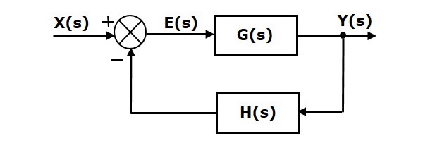
The output of the summing point is -
$$E(s)=X(s)-H(s)Y(s)$$
The output $Y(s)$ is -
$$Y(s)=E(s)G(s)$$
Substitute $E(s)$ value in the above equation.
$$Y(s)=\left \{ X(s)-H(s)Y(s)\rbrace G(s) \right\}$$
$$Y(s)\left \{ 1+G(s)H(s)\rbrace = X(s)G(s) \right\}$$
$$\Rightarrow \frac{Y(s)}{X(s)}=\frac{G(s)}{1+G(s)H(s)}$$
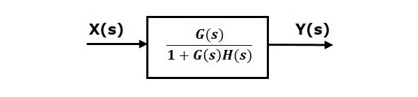
Therefore, the negative feedback closed loop transfer function is $\frac{G(s)}{1+G(s)H(s)}$
This means we can represent the negative feedback connection of two blocks with a single block. The transfer function of this single block is the closed loop transfer function of the negative feedback. The equivalent block diagram is shown below.
Similarly, you can represent the positive feedback connection of two blocks with a single block. The transfer function of this single block is the closed loop transfer function of the positive feedback, i.e., $\frac{G(s)}{1-G(s)H(s)}$
Block Diagram Algebra for Summing Points
There are two possibilities of shifting summing points with respect to blocks −
- Shifting summing point after the block
- Shifting summing point before the block
Let us now see what kind of arrangements need to be done in the above two cases one by one.
Shifting Summing Point After the Block
Consider the block diagram shown in the following figure. Here, the summing point is present before the block.
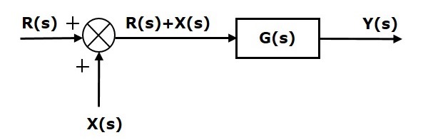
Summing point has two inputs $R(s)$ and $X(s)$. The output of it is $\left \{R(s)+X(s)\right\}$.
So, the input to the block $G(s)$ is $\left \{R(s)+X(s)\right \}$ and the output of it is
$$Y(s)=G(s)\left \{R(s)+X(s)\right \}$$
$\Rightarrow Y(s)=G(s)R(s)+G(s)X(s)$ (Equation 1)
Now, shift the summing point after the block. This block diagram is shown in the following figure.
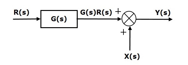
Output of the block $G(s)$ is $G(s)R(s)$.
The output of the summing point is
$Y(s)=G(s)R(s)+X(s)$ (Equation 2)
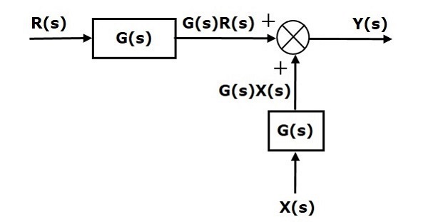
Compare Equation 1 and Equation 2.
The first term $G(s) R(s)$ is same in both the equations. But, there is difference in the second term. In order to get the second term also same, we require one more block $G(s)$. It is having the input $X(s)$ and the output of this block is given as input to summing point instead of $X(s)$. This block diagram is shown in the following figure.
Shifting Summing Point Before the Block
Consider the block diagram shown in the following figure. Here, the summing point is present after the block.
Output of this block diagram is -
$Y(s)=G(s)R(s)+X(s)$ (Equation 3)
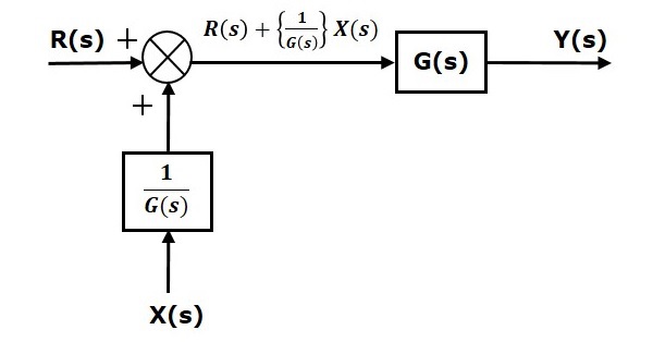
Now, shift the summing point before the block. This block diagram is shown in the following figure.
Output of this block diagram is -
$Y(S)=G(s)R(s)+G(s)X(s)$ (Equation 4)
Compare Equation 3 and Equation 4,
The first term $G(s) R(s)$ is same in both equations. But, there is difference in the second term. In order to get the second term also same, we require one more block $\frac{1}{G(s)}$. It is having the input $X(s)$ and the output of this block is given as input to summing point instead of $X(s)$. This block diagram is shown in the following figure.
Block Diagram Algebra for Take-off Points
There are two possibilities of shifting the take-off points with respect to blocks −
- Shifting take-off point after the block
- Shifting take-off point before the block
Let us now see what kind of arrangements are to be done in the above two cases, one by one.
Shifting Take-off Point After the Block
Consider the block diagram shown in the following figure. In this case, the take-off point is present before the block.
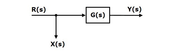
Here, $X(s)=R(s)$ and $Y(s)=G(s)R(s)$
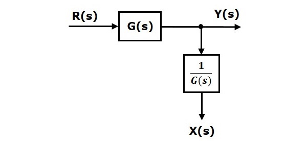
When you shift the take-off point after the block, the output $Y(s)$ will be same. But, there is difference in $X(s)$ value. So, in order to get the same $X(s)$ value, we require one more block $\frac{1}{G(s)}$. It is having the input $Y(s)$ and the output is $X(s)$. This block diagram is shown in the following figure.
Shifting Take-off Point Before the Block
Consider the block diagram shown in the following figure. Here, the take-off point is present after the block.
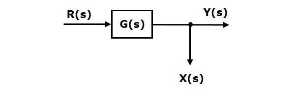
Here, $X(s)=Y(s)=G(s)R(s)$
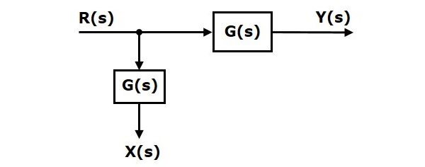
When you shift the take-off point before the block, the output $Y(s)$ will be same. But, there is difference in $X(s)$ value. So, in order to get same $X(s)$ value, we require one more block $G(s)$. It is having the input $R(s)$ and the output is $X(s)$. This block diagram is shown in the following figure.
Control Systems - Block Diagram Reduction
The concepts discussed in the previous chapter are helpful for reducing (simplifying) the block diagrams.
Block Diagram Reduction Rules
Follow these rules for simplifying (reducing) the block diagram, which is having many blocks, summing points and take-off points.
Rule 1 − Check for the blocks connected in series and simplify.
Rule 2 − Check for the blocks connected in parallel and simplify.
Rule 3 − Check for the blocks connected in feedback loop and simplify.
Rule 4 − If there is difficulty with take-off point while simplifying, shift it towards right.
Rule 5 − If there is difficulty with summing point while simplifying, shift it towards left.
Rule 6 − Repeat the above steps till you get the simplified form, i.e., single block.
Note − The transfer function present in this single block is the transfer function of the overall block diagram.
Example
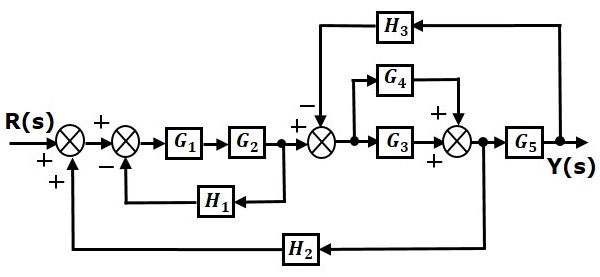
Consider the block diagram shown in the following figure. Let us simplify (reduce) this block diagram using the block diagram reduction rules.
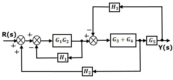
Step 1 − Use Rule 1 for blocks $G_1$ and $G_2$. Use Rule 2 for blocks $G_3$ and $G_4$. The modified block diagram is shown in the following figure.
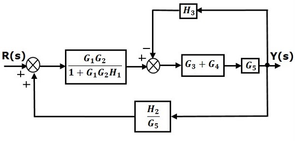
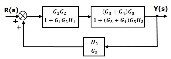
Step 2 − Use Rule 3 for blocks $G_1G_2$ and $H_1$. Use Rule 4 for shifting take-off point after the block $G_5$. The modified block diagram is shown in the following figure.
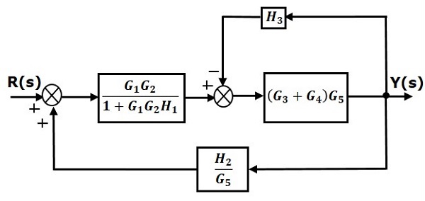
Step 3 − Use Rule 1 for blocks $(G_3 + G_4)$ and $G_5$. The modified block diagram is shown in the following figure.
Step 4 − Use Rule 3 for blocks $(G_3 + G_4)G_5$ and $H_3$. The modified block diagram is shown in the following figure.
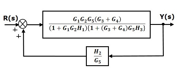
Step 5 − Use Rule 1 for blocks connected in series. The modified block diagram is shown in the following figure.
Step 6 − Use Rule 3 for blocks connected in feedback loop. The modified block diagram is shown in the following figure. This is the simplified block diagram.
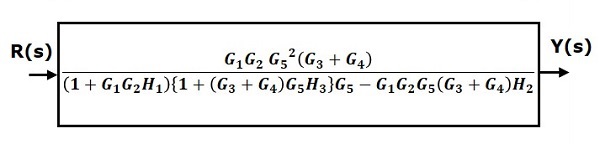
Therefore, the transfer function of the system is
$$\frac{Y(s)}{R(s)}=\frac{G_1G_2G_5^2(G_3+G_4)}{(1+G_1G_2H_1)\lbrace 1+(G_3+G_4)G_5H_3\rbrace G_5-G_1G_2G_5(G_3+G_4)H_2}$$
Note − Follow these steps in order to calculate the transfer function of the block diagram having multiple inputs.
Step 1 − Find the transfer function of block diagram by considering one input at a time and make the remaining inputs as zero.
Step 2 − Repeat step 1 for remaining inputs.
Step 3 − Get the overall transfer function by adding all those transfer functions.
The block diagram reduction process takes more time for complicated systems. Because, we have to draw the (partially simplified) block diagram after each step. So, to overcome this drawback, use signal flow graphs (representation).
In the next two chapters, we will discuss about the concepts related to signal flow graphs, i.e., how to represent signal flow graph from a given block diagram and calculation of transfer function just by using a gain formula without doing any reduction process.
Control Systems - Signal Flow Graphs
Signal flow graph is a graphical representation of algebraic equations. In this chapter, let us discuss the basic concepts related signal flow graph and also learn how to draw signal flow graphs.
Basic Elements of Signal Flow Graph
Nodes and branches are the basic elements of signal flow graph.
Node
Node is a point which represents either a variable or a signal. There are three types of nodes input node, output node and mixed node.
Input Node − It is a node, which has only outgoing branches.
Output Node − It is a node, which has only incoming branches.
Mixed Node − It is a node, which has both incoming and outgoing branches.
Example
Let us consider the following signal flow graph to identify these nodes.
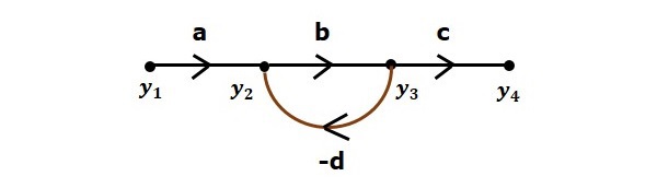
The nodes present in this signal flow graph are y1, y2, y3 and y4.
y1 and y4 are the input node and output node respectively.
y2 and y3 are mixed nodes.
Branch
Branch is a line segment which joins two nodes. It has both gain and direction. For example, there are four branches in the above signal flow graph. These branches have gains of a, b, c and -d.
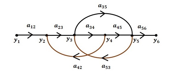
Construction of Signal Flow Graph
Let us construct a signal flow graph by considering the following algebraic equations −
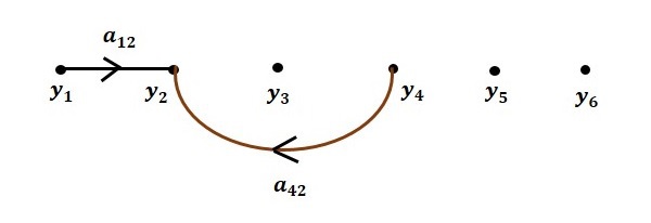
$$y_2=a_{12}y_1+a_{42}y_4$$
$$y_3=a_{23}y_2+a_{53}y_5$$
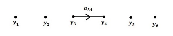
$$y_4=a_{34}y_3$$
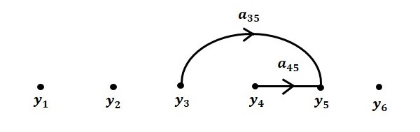
$$y_5=a_{45}y_4+a_{35}y_3$$
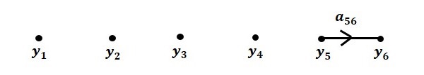
$$y_6=a_{56}y_5$$
There will be six nodes (y1, y2, y3, y4, y5 and y6) and eight branches in this signal flow graph. The gains of the branches are a12, a23, a34, a45, a56, a42, a53 and a35.
To get the overall signal flow graph, draw the signal flow graph for each equation, then combine all these signal flow graphs and then follow the steps given below −
Step 1 − Signal flow graph for $y_2 = a_{13}y_1 + a_{42}y_4$ is shown in the following figure.
Step 2 − Signal flow graph for $y_3 = a_{23}y_2 + a_{53}y_5$ is shown in the following figure.

Step 3 − Signal flow graph for $y_4 = a_{34}y_3$ is shown in the following figure.
Step 4 − Signal flow graph for $y_5 = a_{45}y_4 + a_{35}y_3$ is shown in the following figure.
Step 5 − Signal flow graph for $y_6 = a_{56}y_5$ is shown in the following figure.
Step 6 − Signal flow graph of overall system is shown in the following figure.
Conversion of Block Diagrams into Signal Flow Graphs
Follow these steps for converting a block diagram into its equivalent signal flow graph.
Represent all the signals, variables, summing points and take-off points of block diagram as nodes in signal flow graph.
Represent the blocks of block diagram as branches in signal flow graph.
Represent the transfer functions inside the blocks of block diagram as gains of the branches in signal flow graph.
Connect the nodes as per the block diagram. If there is connection between two nodes (but there is no block in between), then represent the gain of the branch as one. For example, between summing points, between summing point and takeoff point, between input and summing point, between take-off point and output.
Example
Let us convert the following block diagram into its equivalent signal flow graph.
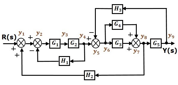
Represent the input signal $R(s)$ and output signal $C(s)$ of block diagram as input node $R(s)$ and output node $C(s)$ of signal flow graph.
Just for reference, the remaining nodes (y1 to y9) are labelled in the block diagram. There are nine nodes other than input and output nodes. That is four nodes for four summing points, four nodes for four take-off points and one node for the variable between blocks $G_1$ and $G_2$.
The following figure shows the equivalent signal flow graph.
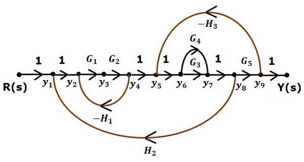
With the help of Masons gain formula (discussed in the next chapter), you can calculate the transfer function of this signal flow graph. This is the advantage of signal flow graphs. Here, we no need to simplify (reduce) the signal flow graphs for calculating the transfer function.
Mason's Gain Formula
Let us now discuss the Masons Gain Formula. Suppose there are N forward paths in a signal flow graph. The gain between the input and the output nodes of a signal flow graph is nothing but the transfer function of the system. It can be calculated by using Masons gain formula.
Masons gain formula is
$$T=\frac{C(s)}{R(s)}=\frac{\Sigma ^N _{i=1}P_i\Delta _i}{\Delta}$$
Where,
C(s) is the output node
R(s) is the input node
T is the transfer function or gain between $R(s)$ and $C(s)$
Pi is the ith forward path gain
$\Delta =1-(sum \: of \: all \: individual \: loop \: gains)$
$+(sum \: of \: gain \: products \: of \: all \: possible \: two \:nontouching \: loops)$
$$-(sum \: of \: gain \: products \: of \: all \: possible \: three \: nontouching \: loops)+...$$
Δi is obtained from Δ by removing the loops which are touching the ith forward path.
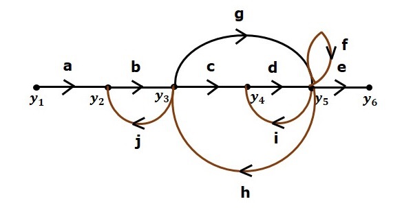
Consider the following signal flow graph in order to understand the basic terminology involved here.
Path
It is a traversal of branches from one node to any other node in the direction of branch arrows. It should not traverse any node more than once.
Examples − $y_2 \rightarrow y_3 \rightarrow y_4 \rightarrow y_5$ and $y_5 \rightarrow y_3 \rightarrow y_2$
Forward Path
The path that exists from the input node to the output node is known as forward path.
Examples − $y_1 \rightarrow y_2 \rightarrow y_3 \rightarrow y_4 \rightarrow y_5 \rightarrow y_6$ and $y_1 \rightarrow y_2 \rightarrow y_3 \rightarrow y_5 \rightarrow y_6$.
Forward Path Gain
It is obtained by calculating the product of all branch gains of the forward path.
Examples − $abcde$ is the forward path gain of $y_1 \rightarrow y_2 \rightarrow y_3 \rightarrow y_4 \rightarrow y_5 \rightarrow y_6$ and abge is the forward path gain of $y_1 \rightarrow y_2 \rightarrow y_3 \rightarrow y_5 \rightarrow y_6$.
Loop
The path that starts from one node and ends at the same node is known as loop. Hence, it is a closed path.
Examples − $y_2 \rightarrow y_3 \rightarrow y_2$ and $y_3 \rightarrow y_5 \rightarrow y_3$.
Loop Gain
It is obtained by calculating the product of all branch gains of a loop.
Examples − $b_j$ is the loop gain of $y_2 \rightarrow y_3 \rightarrow y_2$ and $g_h$ is the loop gain of $y_3 \rightarrow y_5 \rightarrow y_3$.
Non-touching Loops
These are the loops, which should not have any common node.
Examples − The loops, $y_2 \rightarrow y_3 \rightarrow y_2$ and $y_4 \rightarrow y_5 \rightarrow y_4$ are non-touching.
Calculation of Transfer Function using Masons Gain Formula
Let us consider the same signal flow graph for finding transfer function.
Number of forward paths, N = 2.
First forward path is - $y_1 \rightarrow y_2 \rightarrow y_3 \rightarrow y_4 \rightarrow y_5 \rightarrow y_6$.
First forward path gain, $p_1 = abcde$.
Second forward path is - $y_1 \rightarrow y_2 \rightarrow y_3 \rightarrow y_5 \rightarrow y_6$.
Second forward path gain, $p_2 = abge$.
Number of individual loops, L = 5.
Loops are - $y_2 \rightarrow y_3 \rightarrow y_2$, $y_3 \rightarrow y_5 \rightarrow y_3$, $y_3 \rightarrow y_4 \rightarrow y_5 \rightarrow y_3$, $y_4 \rightarrow y_5 \rightarrow y_4$ and $y_5 \rightarrow y_5$.
Loop gains are - $l_1 = bj$, $l_2 = gh$, $l_3 = cdh$, $l_4 = di$ and $l_5 = f$.
Number of two non-touching loops = 2.
First non-touching loops pair is - $y_2 \rightarrow y_3 \rightarrow y_2$, $y_4 \rightarrow y_5 \rightarrow y_4$.
Gain product of first non-touching loops pair, $l_1l_4 = bjdi$
Second non-touching loops pair is - $y_2 \rightarrow y_3 \rightarrow y_2$, $y_5 \rightarrow y_5$.
Gain product of second non-touching loops pair is - $l_1l_5 = bjf$
Higher number of (more than two) non-touching loops are not present in this signal flow graph.
We know,
$\Delta =1-(sum \: of \: all \: individual \: loop \: gains)$
$+(sum \: of \: gain \: products \: of \: all \: possible \: two \:nontouching \: loops)$
$$-(sum \: of \: gain \: products \: of \: all \: possible \: three \: nontouching \: loops)+...$$
Substitute the values in the above equation,
$\Delta =1-(bj+gh+cdh+di+f)+(bjdi+bjf)-(0)$
$\Rightarrow \Delta=1-(bj+gh+cdh+di+f)+bjdi+bjf$
There is no loop which is non-touching to the first forward path.
So, $\Delta_1=1$.
Similarly, $\Delta_2=1$. Since, no loop which is non-touching to the second forward path.
Substitute, N = 2 in Masons gain formula
$$T=\frac{C(s)}{R(s)}=\frac{\Sigma ^2 _{i=1}P_i\Delta _i}{\Delta}$$
$$T=\frac{C(s)}{R(s)}=\frac{P_1\Delta_1+P_2\Delta_2}{\Delta}$$
Substitute all the necessary values in the above equation.
$$T=\frac{C(s)}{R(s)}=\frac{(abcde)1+(abge)1}{1-(bj+gh+cdh+di+f)+bjdi+bjf}$$
$$\Rightarrow T=\frac{C(s)}{R(s)}=\frac{(abcde)+(abge)}{1-(bj+gh+cdh+di+f)+bjdi+bjf}$$
Therefore, the transfer function is -
$$T=\frac{C(s)}{R(s)}=\frac{(abcde)+(abge)}{1-(bj+gh+cdh+di+f)+bjdi+bjf}$$
Control Systems - Time Response Analysis
We can analyze the response of the control systems in both the time domain and the frequency domain. We will discuss frequency response analysis of control systems in later chapters. Let us now discuss about the time response analysis of control systems.
What is Time Response?
If the output of control system for an input varies with respect to time, then it is called the time response of the control system. The time response consists of two parts.
- Transient response
- Steady state response
The response of control system in time domain is shown in the following figure.
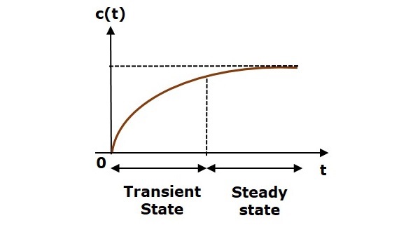
Here, both the transient and the steady states are indicated in the figure. The responses corresponding to these states are known as transient and steady state responses.
Mathematically, we can write the time response c(t) as
$$c(t)=c_{tr}(t)+c_{ss}(t)$$
Where,
- ctr(t) is the transient response
- css(t) is the steady state response
Transient Response
After applying input to the control system, output takes certain time to reach steady state. So, the output will be in transient state till it goes to a steady state. Therefore, the response of the control system during the transient state is known as transient response.
The transient response will be zero for large values of t. Ideally, this value of t is infinity and practically, it is five times constant.
Mathematically, we can write it as
$$\lim_{t\rightarrow \infty }c_{tr}(t)=0$$
Steady state Response
The part of the time response that remains even after the transient response has zero value for large values of t is known as steady state response. This means, the transient response will be zero even during the steady state.
Example
Let us find the transient and steady state terms of the time response of the control system $c(t)=10+5e^{-t}$
Here, the second term $5e^{-t}$ will be zero as t denotes infinity. So, this is the transient term. And the first term 10 remains even as t approaches infinity. So, this is the steady state term.
Standard Test Signals
The standard test signals are impulse, step, ramp and parabolic. These signals are used to know the performance of the control systems using time response of the output.
Unit Impulse Signal
A unit impulse signal, δ(t) is defined as
$\delta (t)=0$ for $t\neq 0$
and $\int_{0^-}^{0^+} \delta (t)dt=1$
The following figure shows unit impulse signal.
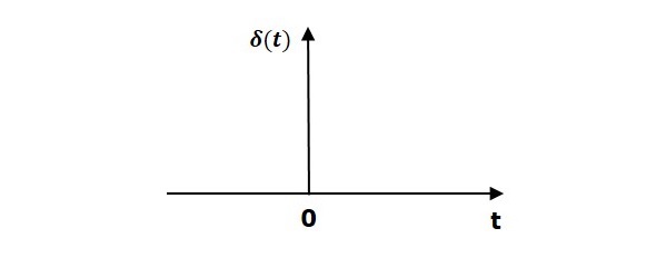
So, the unit impulse signal exists only at t is equal to zero. The area of this signal under small interval of time around t is equal to zero is one. The value of unit impulse signal is zero for all other values of t.
Unit Step Signal
A unit step signal, u(t) is defined as
$$u(t)=1;t\geq 0$$
$=0; t<0$
Following figure shows unit step signal.
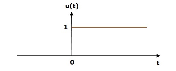
So, the unit step signal exists for all positive values of t including zero. And its value is one during this interval. The value of the unit step signal is zero for all negative values of t.
Unit Ramp Signal
A unit ramp signal, r(t) is defined as
$$r(t)=t; t\geq 0$$
$=0; t<0$
We can write unit ramp signal, $r(t)$ in terms of unit step signal, $u(t)$ as
$$r(t)=tu(t)$$
Following figure shows unit ramp signal.
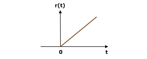
So, the unit ramp signal exists for all positive values of t including zero. And its value increases linearly with respect to t during this interval. The value of unit ramp signal is zero for all negative values of t.
Unit Parabolic Signal
A unit parabolic signal, p(t) is defined as,
$$p(t)=\frac{t^2}{2}; t\geq 0$$
$=0; t<0$
We can write unit parabolic signal, $p(t)$ in terms of the unit step signal, $u(t)$ as,
$$p(t)=\frac{t^2}{2}u(t)$$
The following figure shows the unit parabolic signal.
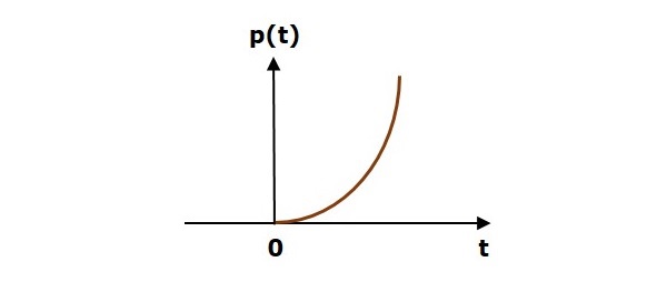
So, the unit parabolic signal exists for all the positive values of t including zero. And its value increases non-linearly with respect to t during this interval. The value of the unit parabolic signal is zero for all the negative values of t.
Response of the First Order System
In this chapter, let us discuss the time response of the first order system. Consider the following block diagram of the closed loop control system. Here, an open loop transfer function, $\frac{1}{sT}$ is connected with a unity negative feedback.
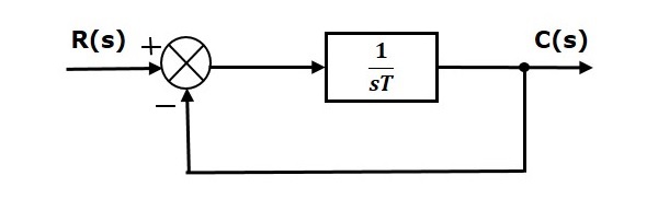
We know that the transfer function of the closed loop control system has unity negative feedback as,
$$\frac{C(s)}{R(s)}=\frac{G(s)}{1+G(s)}$$
Substitute, $G(s)=\frac{1}{sT}$ in the above equation.
$$\frac{C(s)}{R(s)}=\frac{\frac{1}{sT}}{1+\frac{1}{sT}}=\frac{1}{sT+1}$$
The power of s is one in the denominator term. Hence, the above transfer function is of the first order and the system is said to be the first order system.
We can re-write the above equation as
$$C(s)=\left ( \frac{1}{sT+1} \right )R(s)$$
Where,
C(s) is the Laplace transform of the output signal c(t),
R(s) is the Laplace transform of the input signal r(t), and
T is the time constant.
Follow these steps to get the response (output) of the first order system in the time domain.
Take the Laplace transform of the input signal $r(t)$.
Consider the equation, $C(s)=\left ( \frac{1}{sT+1} \right )R(s)$
Substitute $R(s)$ value in the above equation.
Do partial fractions of $C(s)$ if required.
Apply inverse Laplace transform to $C(s)$.
In the previous chapter, we have seen the standard test signals like impulse, step, ramp and parabolic. Let us now find out the responses of the first order system for each input, one by one. The name of the response is given as per the name of the input signal. For example, the response of the system for an impulse input is called as impulse response.
Impulse Response of First Order System
Consider the unit impulse signal as an input to the first order system.
So, $r(t)=\delta (t)$
Apply Laplace transform on both the sides.
$R(s)=1$
Consider the equation, $C(s)=\left ( \frac{1}{sT+1} \right )R(s)$
Substitute, $R(s) = 1$ in the above equation.
$$C(s)=\left ( \frac{1}{sT+1} \right )(1)=\frac{1}{sT+1}$$
Rearrange the above equation in one of the standard forms of Laplace transforms.
$$C(s)=\frac{1}{T\left (\ s+\frac{1}{T} \right )} \Rightarrow C(s)=\frac{1}{T}\left ( \frac{1}{s+\frac{1}{T}} \right )$$
Apply inverse Laplace transform on both sides.
$$c(t)=\frac{1}{T}e^\left ( {-\frac{t}{T}} \right )u(t)$$
The unit impulse response is shown in the following figure.
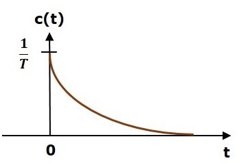
The unit impulse response, c(t) is an exponential decaying signal for positive values of t and it is zero for negative values of t.
Step Response of First Order System
Consider the unit step signal as an input to first order system.
So, $r(t)=u(t)$
Apply Laplace transform on both the sides.
$$R(s)=\frac{1}{s}$$
Consider the equation, $C(s)=\left ( \frac{1}{sT+1} \right )R(s)$
Substitute, $R(s)=\frac{1}{s}$ in the above equation.
$$C(s)=\left ( \frac{1}{sT+1} \right )\left ( \frac{1}{s} \right )=\frac{1}{s\left ( sT+1 \right )}$$
Do partial fractions of C(s).
$$C(s)=\frac{1}{s\left ( sT+1 \right )}=\frac{A}{s}+\frac{B}{sT+1}$$
$$\Rightarrow \frac{1}{s\left ( sT+1 \right )}=\frac{A\left ( sT+1 \right )+Bs}{s\left ( sT+1 \right )}$$
On both the sides, the denominator term is the same. So, they will get cancelled by each other. Hence, equate the numerator terms.
$$1=A\left ( sT+1 \right )+Bs$$
By equating the constant terms on both the sides, you will get A = 1.
Substitute, A = 1 and equate the coefficient of the s terms on both the sides.
$$0=T+B \Rightarrow B=-T$$
Substitute, A = 1 and B = T in partial fraction expansion of $C(s)$.
$$C(s)=\frac{1}{s}-\frac{T}{sT+1}=\frac{1}{s}-\frac{T}{T\left ( s+\frac{1}{T} \right )}$$
$$\Rightarrow C(s)=\frac{1}{s}-\frac{1}{s+\frac{1}{T}}$$
Apply inverse Laplace transform on both the sides.
$$c(t)=\left ( 1-e^{-\left ( \frac{t}{T} \right )} \right )u(t)$$
The unit step response, c(t) has both the transient and the steady state terms.
The transient term in the unit step response is -
$$c_{tr}(t)=-e^{-\left ( \frac{t}{T} \right )}u(t)$$
The steady state term in the unit step response is -
$$c_{ss}(t)=u(t)$$
The following figure shows the unit step response.
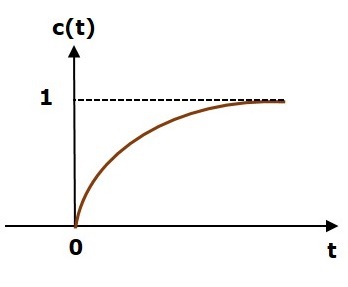
The value of the unit step response, c(t) is zero at t = 0 and for all negative values of t. It is gradually increasing from zero value and finally reaches to one in steady state. So, the steady state value depends on the magnitude of the input.
Ramp Response of First Order System
Consider the unit ramp signal as an input to the first order system.
$So, r(t)=tu(t)$
Apply Laplace transform on both the sides.
$$R(s)=\frac{1}{s^2}$$
Consider the equation, $C(s)=\left ( \frac{1}{sT+1} \right )R(s)$
Substitute, $R(s)=\frac{1}{s^2}$ in the above equation.
$$C(s)=\left ( \frac{1}{sT+1} \right )\left ( \frac{1}{s^2} \right )=\frac{1}{s^2(sT+1)}$$
Do partial fractions of $C(s)$.
$$C(s)=\frac{1}{s^2(sT+1)}=\frac{A}{s^2}+\frac{B}{s}+\frac{C}{sT+1}$$
$$\Rightarrow \frac{1}{s^2(sT+1)}=\frac{A(sT+1)+Bs(sT+1)+Cs^2}{s^2(sT+1)}$$
On both the sides, the denominator term is the same. So, they will get cancelled by each other. Hence, equate the numerator terms.
$$1=A(sT+1)+Bs(sT+1)+Cs^2$$
By equating the constant terms on both the sides, you will get A = 1.
Substitute, A = 1 and equate the coefficient of the s terms on both the sides.
$$0=T+B \Rightarrow B=-T$$
Similarly, substitute B = T and equate the coefficient of $s^2$ terms on both the sides. You will get $C=T^2$.
Substitute A = 1, B = T and $C = T^2$ in the partial fraction expansion of $C(s)$.
$$C(s)=\frac{1}{s^2}-\frac{T}{s}+\frac{T^2}{sT+1}=\frac{1}{s^2}-\frac{T}{s}+\frac{T^2}{T\left ( s+\frac{1}{T} \right )}$$
$$\Rightarrow C(s)=\frac{1}{s^2}-\frac{T}{s}+\frac{T}{s+\frac{1}{T}}$$
Apply inverse Laplace transform on both the sides.
$$c(t)=\left ( t-T+Te^{-\left ( \frac{t}{T} \right )} \right )u(t)$$
The unit ramp response, c(t) has both the transient and the steady state terms.
The transient term in the unit ramp response is -
$$c_{tr}(t)=Te^{-\left ( \frac{t}{T} \right )}u(t)$$
The steady state term in the unit ramp response is -
$$c_{ss}(t)=(t-T)u(t)$$
The following figure shows the unit ramp response.

The unit ramp response, c(t) follows the unit ramp input signal for all positive values of t. But, there is a deviation of T units from the input signal.
Parabolic Response of First Order System
Consider the unit parabolic signal as an input to the first order system.
So, $r(t)=\frac{t^2}{2}u(t)$
Apply Laplace transform on both the sides.
$$R(s)=\frac{1}{s^3}$$
Consider the equation, $C(s)=\left ( \frac{1}{sT+1} \right )R(s)$
Substitute $R(s)=\frac{1}{s^3}$ in the above equation.
$$C(s)=\left ( \frac{1}{sT+1} \right )\left( \frac{1}{s^3} \right )=\frac{1}{s^3(sT+1)}$$
Do partial fractions of $C(s)$.
$$C(s)=\frac{1}{s^3(sT+1)}=\frac{A}{s^3}+\frac{B}{s^2}+\frac{C}{s}+\frac{D}{sT+1}$$
After simplifying, you will get the values of A, B, C and D as 1, $-T, \: T^2\: and \: T^3$ respectively. Substitute these values in the above partial fraction expansion of C(s).
$C(s)=\frac{1}{s^3}-\frac{T}{s^2}+\frac{T^2}{s}-\frac{T^3}{sT+1} \: \Rightarrow C(s)=\frac{1}{s^3}-\frac{T}{s^2}+\frac{T^2}{s}-\frac{T^2}{s+\frac{1}{T}}$
Apply inverse Laplace transform on both the sides.
$$c(t)=\left ( \frac{t^2}{2} -Tt+T^2-T^2e^{-\left ( \frac{t}{T} \right )} \right )u(t)$$
The unit parabolic response, c(t) has both the transient and the steady state terms.
The transient term in the unit parabolic response is
$$C_{tr}(t)=-T^2e^{-\left ( \frac{t}{T} \right )}u(t)$$
The steady state term in the unit parabolic response is
$$C_{ss}(t)=\left ( \frac{t^2}{2} -Tt+T^2 \right )u(t)$$
From these responses, we can conclude that the first order control systems are not stable with the ramp and parabolic inputs because these responses go on increasing even at infinite amount of time. The first order control systems are stable with impulse and step inputs because these responses have bounded output. But, the impulse response doesnt have steady state term. So, the step signal is widely used in the time domain for analyzing the control systems from their responses.
Response of Second Order System
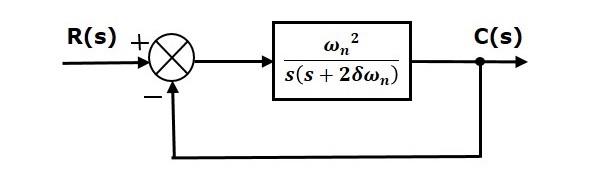
In this chapter, let us discuss the time response of second order system. Consider the following block diagram of closed loop control system. Here, an open loop transfer function, $\frac{\omega ^2_n}{s(s+2\delta \omega_n)}$ is connected with a unity negative feedback.
We know that the transfer function of the closed loop control system having unity negative feedback as
$$\frac{C(s)}{R(s)}=\frac{G(s)}{1+G(s)}$$
Substitute, $G(s)=\frac{\omega ^2_n}{s(s+2\delta \omega_n)}$ in the above equation.
$$\frac{C(s)}{R(s)}=\frac{\left (\frac{\omega ^2_n}{s(s+2\delta \omega_n)} \right )}{1+ \left ( \frac{\omega ^2_n}{s(s+2\delta \omega_n)} \right )}=\frac{\omega _n^2}{s^2+2\delta \omega _ns+\omega _n^2}$$
The power of s is two in the denominator term. Hence, the above transfer function is of the second order and the system is said to be the second order system.
The characteristic equation is -
$$s^2+2\delta \omega _ns+\omega _n^2=0$$
The roots of characteristic equation are -
$$s=\frac{-2\omega \delta _n\pm \sqrt{(2\delta\omega _n)^2-4\omega _n^2}}{2}=\frac{-2(\delta\omega _n\pm \omega _n\sqrt{\delta ^2-1})}{2}$$
$$\Rightarrow s=-\delta \omega_n \pm \omega _n\sqrt{\delta ^2-1}$$
- The two roots are imaginary when δ = 0.
- The two roots are real and equal when δ = 1.
- The two roots are real but not equal when δ > 1.
- The two roots are complex conjugate when 0 < δ < 1.
We can write $C(s)$ equation as,
$$C(s)=\left ( \frac{\omega _n^2}{s^2+2\delta\omega_ns+\omega_n^2} \right )R(s)$$
Where,
C(s) is the Laplace transform of the output signal, c(t)
R(s) is the Laplace transform of the input signal, r(t)
ωn is the natural frequency
δ is the damping ratio.
Follow these steps to get the response (output) of the second order system in the time domain.
Take Laplace transform of the input signal, $r(t)$.
Consider the equation, $C(s)=\left ( \frac{\omega _n^2}{s^2+2\delta\omega_ns+\omega_n^2} \right )R(s)$
Substitute $R(s)$ value in the above equation.
Do partial fractions of $C(s)$ if required.
Apply inverse Laplace transform to $C(s)$.
Step Response of Second Order System
Consider the unit step signal as an input to the second order system.
Laplace transform of the unit step signal is,
$$R(s)=\frac{1}{s}$$
We know the transfer function of the second order closed loop control system is,
$$\frac{C(s)}{R(s)}=\frac{\omega _n^2}{s^2+2\delta\omega_ns+\omega_n^2}$$
Case 1: δ = 0
Substitute, $\delta = 0$ in the transfer function.
$$\frac{C(s)}{R(s)}=\frac{\omega_n^2}{s^2+\omega_n^2}$$
$$\Rightarrow C(s)=\left( \frac{\omega_n^2}{s^2+\omega_n^2} \right )R(s)$$
Substitute, $R(s) = \frac{1}{s}$ in the above equation.
$$C(s)=\left( \frac{\omega_n^2}{s^2+\omega_n^2} \right )\left( \frac{1}{s} \right )=\frac{\omega_n^2}{s(s^2+\omega_n^2)}$$
Apply inverse Laplace transform on both the sides.
$$c(t)=\left ( 1-\cos(\omega_n t) \right )u(t)$$
So, the unit step response of the second order system when $/delta = 0$ will be a continuous time signal with constant amplitude and frequency.
Case 2: δ = 1
Substitute, $/delta = 1$ in the transfer function.
$$\frac{C(s)}{R(s)}=\frac{\omega_n^2}{s^2+2\omega_ns+\omega_n^2}$$
$$\Rightarrow C(s)=\left( \frac{\omega_n^2}{(s+\omega_n)^2} \right)R(s)$$
Substitute, $R(s) = \frac{1}{s}$ in the above equation.
$$C(s)=\left( \frac{\omega_n^2}{(s+\omega_n)^2} \right)\left ( \frac{1}{s} \right)=\frac{\omega_n^2}{s(s+\omega_n)^2}$$
Do partial fractions of $C(s)$.
$$C(s)=\frac{\omega_n^2}{s(s+\omega_n)^2}=\frac{A}{s}+\frac{B}{s+\omega_n}+\frac{C}{(s+\omega_n)^2}$$
After simplifying, you will get the values of A, B and C as $1,\: -1\: and \: \omega _n$ respectively. Substitute these values in the above partial fraction expansion of $C(s)$.
$$C(s)=\frac{1}{s}-\frac{1}{s+\omega_n}-\frac{\omega_n}{(s+\omega_n)^2}$$
Apply inverse Laplace transform on both the sides.
$$c(t)=(1-e^{-\omega_nt}-\omega _nte^{-\omega_nt})u(t)$$
So, the unit step response of the second order system will try to reach the step input in steady state.
Case 3: 0 < δ < 1
We can modify the denominator term of the transfer function as follows −
$$s^2+2\delta\omega_ns+\omega_n^2=\left \{ s^2+2(s)(\delta \omega_n)+(\delta \omega_n)^2 \right \}+\omega_n^2-(\delta\omega_n)^2$$
$$=(s+\delta\omega_n)^2+\omega_n^2(1-\delta^2)$$
The transfer function becomes,
$$\frac{C(s)}{R(s)}=\frac{\omega_n^2}{(s+\delta\omega_n)^2+\omega_n^2(1-\delta^2)}$$
$$\Rightarrow C(s)=\left( \frac{\omega_n^2}{(s+\delta\omega_n)^2+\omega_n^2(1-\delta^2)} \right )R(s)$$
Substitute, $R(s) = \frac{1}{s}$ in the above equation.
$$C(s)=\left( \frac{\omega_n^2}{(s+\delta\omega_n)^2+\omega_n^2(1-\delta^2)} \right )\left( \frac{1}{s} \right )=\frac{\omega_n^2}{s\left ((s+\delta\omega_n)^2+\omega_n^2(1-\delta^2) \right)}$$
Do partial fractions of $C(s)$.
$$C(s)=\frac{\omega_n^2}{s\left ((s+\delta\omega_n)^2+\omega_n^2(1-\delta^2) \right)}=\frac{A}{s}+\frac{Bs+C}{(s+\delta\omega_n)^2+\omega_n^2(1-\delta^2)}$$
After simplifying, you will get the values of A, B and C as $1,\: -1 \: and \: 2\delta \omega _n$ respectively. Substitute these values in the above partial fraction expansion of C(s).
$$C(s)=\frac{1}{s}-\frac{s+2\delta\omega_n}{(s+\delta\omega_n)^2+\omega_n^2(1-\delta^2)}$$
$$C(s)=\frac{1}{s}-\frac{s+\delta\omega_n}{(s+\delta\omega_n)^2+\omega_n^2(1-\delta^2)}-\frac{\delta\omega_n}{(s+\delta\omega_n)^2+\omega_n^2(1-\delta^2)}$$
$C(s)=\frac{1}{s}-\frac{(s+\delta\omega_n)}{(s+\delta\omega_n)^2+(\omega_n\sqrt{1-\delta^2})^2}-\frac{\delta}{\sqrt{1-\delta^2}}\left ( \frac{\omega_n\sqrt{1-\delta^2}}{(s+\delta\omega_n)^2+(\omega_n\sqrt{1-\delta^2})^2} \right )$
Substitute, $\omega_n\sqrt{1-\delta^2}$ as $\omega_d$ in the above equation.
$$C(s)=\frac{1}{s}-\frac{(s+\delta\omega_n)}{(s+\delta\omega_n)^2+\omega_d^2}-\frac{\delta}{\sqrt{1-\delta^2}}\left ( \frac{\omega_d}{(s+\delta\omega_n)^2+\omega_d^2} \right )$$
Apply inverse Laplace transform on both the sides.
$$c(t)=\left ( 1-e^{-\delta \omega_nt}\cos(\omega_dt)-\frac{\delta}{\sqrt{1-\delta^2}}e^{-\delta\omega_nt}\sin(\omega_dt) \right )u(t)$$
$$c(t)=\left ( 1-\frac{e^{-\delta\omega_nt}}{\sqrt{1-\delta^2}}\left ( (\sqrt{1-\delta^2})\cos(\omega_dt)+\delta \sin(\omega_dt) \right ) \right )u(t)$$
If $\sqrt{1-\delta^2}=\sin(\theta)$, then δ will be cos(θ). Substitute these values in the above equation.
$$c(t)=\left ( 1-\frac{e^{-\delta\omega_nt}}{\sqrt{1-\delta^2}}(\sin(\theta)\cos(\omega_dt)+\cos(\theta)\sin(\omega_dt)) \right )u(t)$$
$$\Rightarrow c(t)=\left ( 1-\left ( \frac{e^{-\delta\omega_nt}}{\sqrt{1-\delta^2}} \right )\sin(\omega_dt+\theta) \right )u(t)$$
So, the unit step response of the second order system is having damped oscillations (decreasing amplitude) when δ lies between zero and one.
Case 4: δ > 1
We can modify the denominator term of the transfer function as follows −
$$s^2+2\delta\omega_ns+\omega_n^2=\left \{ s^2+2(s)(\delta\omega_n)+(\delta\omega_n)^2 \right \}+\omega_n^2-(\delta\omega_n)^2$$
$$=\left ( s+\delta\omega_n \right )^2-\omega_n^2\left ( \delta^2-1 \right )$$
The transfer function becomes,
$$\frac{C(s)}{R(s)}=\frac{\omega_n^2}{(s+\delta\omega_n)^2-\omega_n^2(\delta^2-1)}$$
$$\Rightarrow C(s)=\left ( \frac{\omega_n^2}{(s+\delta\omega_n)^2-\omega_n^2(\delta^2-1)} \right )R(s)$$
Substitute, $R(s) = \frac{1}{s}$ in the above equation.
$C(s)=\left ( \frac{\omega_n^2}{(s+\delta\omega_n)^2-(\omega_n\sqrt{\delta^2-1})^2} \right )\left ( \frac{1}{s} \right )=\frac{\omega_n^2}{s(s+\delta\omega_n+\omega_n\sqrt{\delta^2-1})(s+\delta\omega_n-\omega_n\sqrt{\delta^2-1})}$
Do partial fractions of $C(s)$.
$$C(s)=\frac{\omega_n^2}{s(s+\delta\omega_n+\omega_n\sqrt{\delta^2-1})(s+\delta\omega_n-\omega_n\sqrt{\delta^2-1})}$$
$$=\frac{A}{s}+\frac{B}{s+\delta\omega_n+\omega_n\sqrt{\delta^2-1}}+\frac{C}{s+\delta\omega_n-\omega_n\sqrt{\delta^2-1}}$$
After simplifying, you will get the values of A, B and C as 1, $\frac{1}{2(\delta+\sqrt{\delta^2-1})(\sqrt{\delta^2-1})}$ and $\frac{-1}{2(\delta-\sqrt{\delta^2-1})(\sqrt{\delta^2-1})}$ respectively. Substitute these values in above partial fraction expansion of $C(s)$.
$$C(s)=\frac{1}{s}+\frac{1}{2(\delta+\sqrt{\delta^2-1})(\sqrt{\delta^2-1})}\left ( \frac{1}{s+\delta\omega_n+\omega_n\sqrt{\delta^2-1}} \right )-\left ( \frac{1}{2(\delta-\sqrt{\delta^2-1})(\sqrt{\delta^2-1})} \right )\left ( \frac{1}{s+\delta\omega_n-\omega_n\sqrt{\delta^2-1}} \right )$$
Apply inverse Laplace transform on both the sides.
$c(t)=\left ( 1+\left ( \frac{1}{2(\delta+\sqrt{\delta^2-1})(\sqrt{\delta^2-1})} \right )e^{-(\delta\omega_n+\omega_n\sqrt{\delta^2-1})t}-\left ( \frac{1}{2(\delta-\sqrt{\delta^2-1})(\sqrt{\delta^2-1})} \right )e^{-(\delta\omega_n-\omega_n\sqrt{\delta^2-1})t} \right )u(t)$
Since it is over damped, the unit step response of the second order system when δ > 1 will never reach step input in the steady state.
Impulse Response of Second Order System
The impulse response of the second order system can be obtained by using any one of these two methods.
Follow the procedure involved while deriving step response by considering the value of $R(s)$ as 1 instead of $\frac{1}{s}$.
Do the differentiation of the step response.
The following table shows the impulse response of the second order system for 4 cases of the damping ratio.
| Condition of Damping ratio | Impulse response for t ≥ 0 |
|---|---|
δ = 0 |
$\omega_n\sin(\omega_nt)$ |
δ = 1 |
$\omega_n^2te^{-\omega_nt}$ |
0 < δ < 1 |
$\left ( \frac{\omega_ne^{-\delta\omega_nt}}{\sqrt{1-\delta^2}} \right )\sin(\omega_dt)$ |
δ > 1 |
$\left ( \frac{\omega_n}{2\sqrt{\delta^2-1}} \right )\left ( e^{-(\delta\omega_n-\omega_n\sqrt{\delta^2-1})t}-e^{-(\delta\omega_n+\omega_n\sqrt{\delta^2-1})t} \right )$ |
Time Domain Specifications
In this chapter, let us discuss the time domain specifications of the second order system. The step response of the second order system for the underdamped case is shown in the following figure.
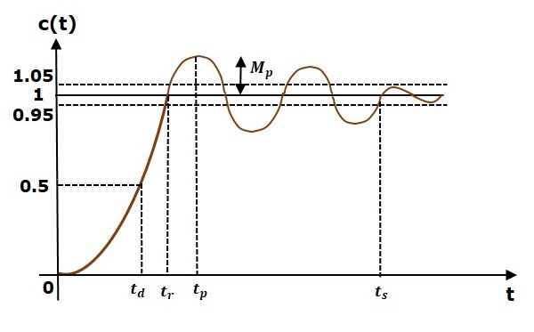
All the time domain specifications are represented in this figure. The response up to the settling time is known as transient response and the response after the settling time is known as steady state response.
Delay Time
It is the time required for the response to reach half of its final value from the zero instant. It is denoted by $t_d$.
Consider the step response of the second order system for t ≥ 0, when δ lies between zero and one.
$$c(t)=1-\left ( \frac{e^{-\delta \omega_nt}}{\sqrt{1-\delta^2}} \right )\sin(\omega_dt+\theta)$$
The final value of the step response is one.
Therefore, at $t=t_d$, the value of the step response will be 0.5. Substitute, these values in the above equation.
$$c(t_d)=0.5=1-\left ( \frac{e^{-\delta\omega_nt_d}}{\sqrt{1-\delta^2}} \right )\sin(\omega_dt_d+\theta)$$
$$\Rightarrow \left ( \frac{e^{-\delta\omega_nt_d}}{\sqrt{1-\delta^2}} \right )\sin(\omega_dt_d+\theta)=0.5$$
By using linear approximation, you will get the delay time td as
$$t_d=\frac{1+0.7\delta}{\omega_n}$$
Rise Time
It is the time required for the response to rise from 0% to 100% of its final value. This is applicable for the under-damped systems. For the over-damped systems, consider the duration from 10% to 90% of the final value. Rise time is denoted by tr.
At t = t1 = 0, c(t) = 0.
We know that the final value of the step response is one.
Therefore, at $t = t_2$, the value of step response is one. Substitute, these values in the following equation.
$$c(t)=1-\left ( \frac{e^{-\delta \omega_nt}}{\sqrt{1-\delta^2}} \right )\sin(\omega_dt+\theta)$$
$$c(t_2)=1=1-\left ( \frac{e^{-\delta\omega_nt_2}}{\sqrt{1-\delta^2}} \right )\sin(\omega_dt_2+\theta)$$
$$\Rightarrow \left ( \frac{e^{-\delta\omega_nt_2}}{\sqrt{1-\delta^2}} \right )\sin(\omega_dt_2+\theta)=0$$
$$\Rightarrow \sin(\omega_dt_2+\theta)=0$$
$$\Rightarrow \omega_dt_2+\theta=\pi$$
$$\Rightarrow t_2=\frac{\pi-\theta}{\omega_d}$$
Substitute t1 and t2 values in the following equation of rise time,
$$t_r=t_2-t_1$$
$$\therefore \: t_r=\frac{\pi-\theta}{\omega_d}$$
From above equation, we can conclude that the rise time $t_r$ and the damped frequency $\omega_d$ are inversely proportional to each other.
Peak Time
It is the time required for the response to reach the peak value for the first time. It is denoted by $t_p$. At $t = t_p$, the first derivate of the response is zero.
We know the step response of second order system for under-damped case is
$$c(t)=1-\left ( \frac{e^{-\delta \omega_nt}}{\sqrt{1-\delta^2}} \right )\sin(\omega_dt+\theta)$$
Differentiate $c(t)$ with respect to t.
$$\frac{\text{d}c(t)}{\text{d}t}=-\left ( \frac{e^{-\delta\omega_nt}}{\sqrt{1-\delta^2}} \right )\omega_d\cos(\omega_dt+\theta)-\left ( \frac{-\delta\omega_ne^{-\delta\omega_nt}}{\sqrt{1-\delta^2}} \right )\sin(\omega_dt+\theta)$$
Substitute, $t=t_p$ and $\frac{\text{d}c(t)}{\text{d}t}=0$ in the above equation.
$$0=-\left ( \frac{e^{-\delta\omega_nt_p}}{\sqrt{1-\delta^2}} \right )\left [ \omega_d\cos(\omega_dt_p+\theta)-\delta\omega_n\sin(\omega_dt_p+\theta) \right ]$$
$$\Rightarrow \omega_n\sqrt{1-\delta^2}\cos(\omega_dt_p+\theta)-\delta\omega_n\sin(\omega_dt_p+\theta)=0$$
$$\Rightarrow \sqrt{1-\delta^2}\cos(\omega_dt_p+\theta)-\delta\sin(\omega_dt_p+\theta)=0$$
$$\Rightarrow \sin(\theta)\cos(\omega_dt_p+\theta)-\cos(\theta)\sin(\omega_dt_p+\theta)=0$$
$$\Rightarrow \sin(\theta-\omega_dt_p-\theta)=0$$
$$\Rightarrow sin(-\omega_dt_p)=0\Rightarrow -\sin(\omega_dt_p)=0\Rightarrow sin(\omega_dt_p)=0$$
$$\Rightarrow \omega_dt_p=\pi$$
$$\Rightarrow t_p=\frac{\pi}{\omega_d}$$
From the above equation, we can conclude that the peak time $t_p$ and the damped frequency $\omega_d$ are inversely proportional to each other.
Peak Overshoot
Peak overshoot Mp is defined as the deviation of the response at peak time from the final value of response. It is also called the maximum overshoot.
Mathematically, we can write it as
$$M_p=c(t_p)-c(\infty)$$
Where,
c(tp) is the peak value of the response.
c(∞) is the final (steady state) value of the response.
At $t = t_p$, the response c(t) is -
$$c(t_p)=1-\left ( \frac{e^{-\delta\omega_nt_p}}{\sqrt{1-\delta^2}} \right )\sin(\omega_dt_p+\theta)$$
Substitute, $t_p=\frac{\pi}{\omega_d}$ in the right hand side of the above equation.
$$c(t_P)=1-\left ( \frac{e^{-\delta\omega_n\left ( \frac{\pi}{\omega_d} \right )}}{\sqrt{1-\delta^2}} \right )\sin\left ( \omega_d\left ( \frac{\pi}{\omega_d} \right ) +\theta\right )$$
$$\Rightarrow c(t_p)=1-\left ( \frac{e^{-\left ( \frac{\delta\pi}{\sqrt{1-\delta^2}} \right )}}{\sqrt{1-\delta^2}} \right )(-\sin(\theta))$$
We know that
$$\sin(\theta)=\sqrt{1-\delta^2}$$
So, we will get $c(t_p)$ as
$$c(t_p)=1+e^{-\left ( \frac{\delta\pi}{\sqrt{1-\delta^2}} \right )}$$
Substitute the values of $c(t_p)$ and $c(\infty)$ in the peak overshoot equation.
$$M_p=1+e^{-\left ( \frac{\delta\pi}{\sqrt{1-\delta^2}} \right )}-1$$
$$\Rightarrow M_p=e^{-\left ( \frac{\delta\pi}{\sqrt{1-\delta^2}} \right )}$$
Percentage of peak overshoot % $M_p$ can be calculated by using this formula.
$$\%M_p=\frac{M_p}{c(\infty )}\times 100\%$$
By substituting the values of $M_p$ and $c(\infty)$ in above formula, we will get the Percentage of the peak overshoot $\%M_p$ as
$$\%M_p=\left ( e^ {-\left ( \frac{\delta\pi}{\sqrt{1-\delta^2}} \right )} \right )\times 100\%$$
From the above equation, we can conclude that the percentage of peak overshoot $\% M_p$ will decrease if the damping ratio $\delta$ increases.
Settling time
It is the time required for the response to reach the steady state and stay within the specified tolerance bands around the final value. In general, the tolerance bands are 2% and 5%. The settling time is denoted by $t_s$.
The settling time for 5% tolerance band is -
$$t_s=\frac{3}{\delta\omega_n}=3\tau$$
The settling time for 2% tolerance band is -
$$t_s=\frac{4}{\delta\omega_n}=4\tau$$
Where, $\tau$ is the time constant and is equal to $\frac{1}{\delta\omega_n}$.
Both the settling time $t_s$ and the time constant $\tau$ are inversely proportional to the damping ratio $\delta$.
Both the settling time $t_s$ and the time constant $\tau$ are independent of the system gain. That means even the system gain changes, the settling time $t_s$ and time constant $\tau$ will never change.
Example
Let us now find the time domain specifications of a control system having the closed loop transfer function $\frac{4}{s^2+2s+4}$ when the unit step signal is applied as an input to this control system.
We know that the standard form of the transfer function of the second order closed loop control system as
$$\frac{\omega_n^2}{s^2+2\delta\omega_ns+\omega_n^2}$$
By equating these two transfer functions, we will get the un-damped natural frequency $\omega_n$ as 2 rad/sec and the damping ratio $\delta$ as 0.5.
We know the formula for damped frequency $\omega_d$ as
$$\omega_d=\omega_n\sqrt{1-\delta^2}$$
Substitute, $\omega_n$ and $\delta$ values in the above formula.
$$\Rightarrow \omega_d=2\sqrt{1-(0.5)^2}$$
$$\Rightarrow \omega_d=1.732 \: rad/sec$$
Substitute, $\delta$ value in following relation
$$\theta=\cos^{-1}\delta$$
$$\Rightarrow \theta=\cos^{-1}(0.5)=\frac{\pi}{3}\:rad$$
Substitute the above necessary values in the formula of each time domain specification and simplify in order to get the values of time domain specifications for given transfer function.
The following table shows the formulae of time domain specifications, substitution of necessary values and the final values.
| Time domain specification | Formula | Substitution of values in Formula | Final value |
|---|---|---|---|
Delay time |
$t_d=\frac{1+0.7\delta}{\omega_n}$ |
$t_d=\frac{1+0.7(0.5)}{2}$ |
$t_d$=0.675 sec |
Rise time |
$t_r=\frac{\pi-\theta}{\omega_d}$ |
$t_r=\frac{\pi-(\frac{\pi}{3})}{1.732}$ |
$t_r$=1.207 sec |
Peak time |
$t_p=\frac{\pi}{\omega_d}$ |
$t_p=\frac{\pi}{1.732}$ |
$t_p$=1.813 sec |
% Peak overshoot |
$\%M_p=\left( e^{-\left (\frac{\delta\pi}{\sqrt{1-\delta^2}} \right ) }\right )\times 100\%$ |
$\%M_p=\left( e^{-\left (\frac{0.5\pi}{\sqrt{1-(0.5)^2}} \right ) }\right )\times 100\%$ |
$\% \: M_p$=16.32% |
Settling time for 2% tolerance band |
$t_s=\frac{4}{\delta\omega_n}$ |
$t_S=\frac{4}{(0.5)(2)}$ |
$t_s$=4 sec |
Control Systems - Steady State Errors
The deviation of the output of control system from desired response during steady state is known as steady state error. It is represented as $e_{ss}$. We can find steady state error using the final value theorem as follows.
$$e_{ss}=\lim_{t \to \infty}e(t)=\lim_{s \to 0}sE(s)$$
Where,
E(s) is the Laplace transform of the error signal, $e(t)$
Let us discuss how to find steady state errors for unity feedback and non-unity feedback control systems one by one.
Steady State Errors for Unity Feedback Systems
Consider the following block diagram of closed loop control system, which is having unity negative feedback.
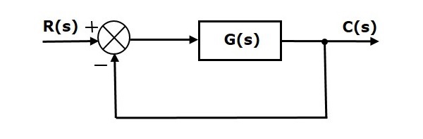
Where,
- R(s) is the Laplace transform of the reference Input signal $r(t)$
- C(s) is the Laplace transform of the output signal $c(t)$
We know the transfer function of the unity negative feedback closed loop control system as
$$\frac{C(s)}{R(s)}=\frac{G(s)}{1+G(s)}$$
$$\Rightarrow C(s)=\frac{R(s)G(s)}{1+G(s)}$$
The output of the summing point is -
$$E(s)=R(s)-C(s)$$
Substitute $C(s)$ value in the above equation.
$$E(s)=R(s)-\frac{R(s)G(s)}{1+G(s)}$$
$$\Rightarrow E(s)=\frac{R(s)+R(s)G(s)-R(s)G(s)}{1+G(s)}$$
$$\Rightarrow E(s)=\frac{R(s)}{1+G(s)}$$
Substitute $E(s)$ value in the steady state error formula
$$e_{ss}=\lim_{s \to 0} \frac{sR(s)}{1+G(s)}$$
The following table shows the steady state errors and the error constants for standard input signals like unit step, unit ramp & unit parabolic signals.
| Input signal | Steady state error $e_{ss}$ | Error constant |
|---|---|---|
unit step signal |
$\frac{1}{1+k_p}$ |
$K_p=\lim_{s \to 0}G(s)$ |
unit ramp signal |
$\frac{1}{K_v}$ |
$K_v=\lim_{s \to 0}sG(s)$ |
unit parabolic signal |
$\frac{1}{K_a}$ |
$K_a=\lim_{s \to 0}s^2G(s)$ |
Where, $K_p$, $K_v$ and $K_a$ are position error constant, velocity error constant and acceleration error constant respectively.
Note − If any of the above input signals has the amplitude other than unity, then multiply corresponding steady state error with that amplitude.
Note − We cant define the steady state error for the unit impulse signal because, it exists only at origin. So, we cant compare the impulse response with the unit impulse input as t denotes infinity.
Example
Let us find the steady state error for an input signal $r(t)=\left( 5+2t+\frac{t^2}{2} \right )u(t)$ of unity negative feedback control system with $G(s)=\frac{5(s+4)}{s^2(s+1)(s+20)}$
The given input signal is a combination of three signals step, ramp and parabolic. The following table shows the error constants and steady state error values for these three signals.
| Input signal | Error constant | Steady state error |
|---|---|---|
$r_1(t)=5u(t)$ |
$K_p=\lim_{s \to 0}G(s)=\infty$ |
$e_{ss1}=\frac{5}{1+k_p}=0$ |
$r_2(t)=2tu(t)$ |
$K_v=\lim_{s \to 0}sG(s)=\infty$ |
$e_{ss2}=\frac{2}{K_v}=0$ |
$r_3(t)=\frac{t^2}{2}u(t)$ |
$K_a=\lim_{s \to 0}s^2G(s)=1$ |
$e_{ss3}=\frac{1}{k_a}=1$ |
We will get the overall steady state error, by adding the above three steady state errors.
$$e_{ss}=e_{ss1}+e_{ss2}+e_{ss3}$$
$$\Rightarrow e_{ss}=0+0+1=1$$
Therefore, we got the steady state error $e_{ss}$ as 1 for this example.
Steady State Errors for Non-Unity Feedback Systems
Consider the following block diagram of closed loop control system, which is having nonunity negative feedback.
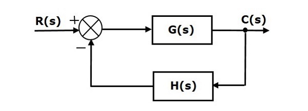
We can find the steady state errors only for the unity feedback systems. So, we have to convert the non-unity feedback system into unity feedback system. For this, include one unity positive feedback path and one unity negative feedback path in the above block diagram. The new block diagram looks like as shown below.
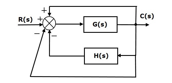
Simplify the above block diagram by keeping the unity negative feedback as it is. The following is the simplified block diagram.
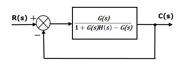
This block diagram resembles the block diagram of the unity negative feedback closed loop control system. Here, the single block is having the transfer function $\frac{G(s)}{1+G(s)H(s)-G(s)}$ instead of $G(s)$. You can now calculate the steady state errors by using steady state error formula given for the unity negative feedback systems.
Note − It is meaningless to find the steady state errors for unstable closed loop systems. So, we have to calculate the steady state errors only for closed loop stable systems. This means we need to check whether the control system is stable or not before finding the steady state errors. In the next chapter, we will discuss the concepts-related stability.
Control Systems - Stability
Stability is an important concept. In this chapter, let us discuss the stability of system and types of systems based on stability.
What is Stability?
A system is said to be stable, if its output is under control. Otherwise, it is said to be unstable. A stable system produces a bounded output for a given bounded input.
The following figure shows the response of a stable system.
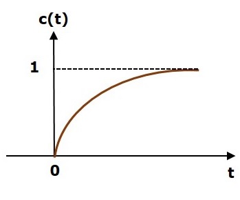
This is the response of first order control system for unit step input. This response has the values between 0 and 1. So, it is bounded output. We know that the unit step signal has the value of one for all positive values of t including zero. So, it is bounded input. Therefore, the first order control system is stable since both the input and the output are bounded.
Types of Systems based on Stability
We can classify the systems based on stability as follows.
- Absolutely stable system
- Conditionally stable system
- Marginally stable system
Absolutely Stable System
If the system is stable for all the range of system component values, then it is known as the absolutely stable system. The open loop control system is absolutely stable if all the poles of the open loop transfer function present in left half of s plane. Similarly, the closed loop control system is absolutely stable if all the poles of the closed loop transfer function present in the left half of the s plane.
Conditionally Stable System
If the system is stable for a certain range of system component values, then it is known as conditionally stable system.
Marginally Stable System
If the system is stable by producing an output signal with constant amplitude and constant frequency of oscillations for bounded input, then it is known as marginally stable system. The open loop control system is marginally stable if any two poles of the open loop transfer function is present on the imaginary axis. Similarly, the closed loop control system is marginally stable if any two poles of the closed loop transfer function is present on the imaginary axis.
Control Systems - Stability Analysis
In this chapter, let us discuss the stability analysis in the s domain using the RouthHurwitz stability criterion. In this criterion, we require the characteristic equation to find the stability of the closed loop control systems.
Routh-Hurwitz Stability Criterion
Routh-Hurwitz stability criterion is having one necessary condition and one sufficient condition for stability. If any control system doesnt satisfy the necessary condition, then we can say that the control system is unstable. But, if the control system satisfies the necessary condition, then it may or may not be stable. So, the sufficient condition is helpful for knowing whether the control system is stable or not.
Necessary Condition for Routh-Hurwitz Stability
The necessary condition is that the coefficients of the characteristic polynomial should be positive. This implies that all the roots of the characteristic equation should have negative real parts.
Consider the characteristic equation of the order n is -
$$a_0s^n+a_1s^{n-1}+a_2s^{n-2}+...+a_{n-1}s^1+a_ns^0=0$$
Note that, there should not be any term missing in the nth order characteristic equation. This means that the nth order characteristic equation should not have any coefficient that is of zero value.
Sufficient Condition for Routh-Hurwitz Stability
The sufficient condition is that all the elements of the first column of the Routh array should have the same sign. This means that all the elements of the first column of the Routh array should be either positive or negative.
Routh Array Method
If all the roots of the characteristic equation exist to the left half of the s plane, then the control system is stable. If at least one root of the characteristic equation exists to the right half of the s plane, then the control system is unstable. So, we have to find the roots of the characteristic equation to know whether the control system is stable or unstable. But, it is difficult to find the roots of the characteristic equation as order increases.
So, to overcome this problem there we have the Routh array method. In this method, there is no need to calculate the roots of the characteristic equation. First formulate the Routh table and find the number of the sign changes in the first column of the Routh table. The number of sign changes in the first column of the Routh table gives the number of roots of characteristic equation that exist in the right half of the s plane and the control system is unstable.
Follow this procedure for forming the Routh table.
Fill the first two rows of the Routh array with the coefficients of the characteristic polynomial as mentioned in the table below. Start with the coefficient of $s^n$ and continue up to the coefficient of $s^0$.
Fill the remaining rows of the Routh array with the elements as mentioned in the table below. Continue this process till you get the first column element of row $s^0$ is $a_n$. Here, $a_n$ is the coefficient of $s^0$ in the characteristic polynomial.
Note − If any row elements of the Routh table have some common factor, then you can divide the row elements with that factor for the simplification will be easy.
The following table shows the Routh array of the nth order characteristic polynomial.
$$a_0s^n+a_1s^{n-1}+a_2s^{n-2}+...+a_{n-1}s^1+a_ns^0$$
$s^n$ |
$a_0$ |
$a_2$ |
$a_4$ |
$a_6$ |
... |
... |
$s^{n-1}$ |
$a_1$ |
$a_3$ |
$a_5$ |
$a_7$ |
... |
... |
$s^{n-2}$ |
$b_1=\frac{a_1a_2-a_3a_0}{a_1}$ |
$b_2=\frac{a_1a_4-a_5a_0}{a_1}$ |
$b_3=\frac{a_1a_6-a_7a_0}{a_1}$ |
... |
... |
... |
$s^{n-3}$ |
$c_1=\frac{b_1a_3-b_2a_1}{b_1}$ |
$c_2=\frac{b_1a_55-b_3a_1}{b_1}$ |
$\vdots$ |
|||
$\vdots $ |
$\vdots$ |
$\vdots$ |
$\vdots$ |
|||
$s^1$ |
$\vdots$ |
$\vdots$ |
||||
$s^0$ |
$a_n$ |
Example
Let us find the stability of the control system having characteristic equation,
$$s^4+3s^3+3s^2+2s+1=0$$
Step 1 − Verify the necessary condition for the Routh-Hurwitz stability.
All the coefficients of the characteristic polynomial, $s^4+3s^3+3s^2+2s+1$ are positive. So, the control system satisfies the necessary condition.
Step 2 − Form the Routh array for the given characteristic polynomial.
$s^4$ |
$1$ |
$3$ |
$1$ |
$s^3$ |
$3$ |
$2$ |
|
$s^2$ |
$\frac{(3 \times 3)-(2 \times 1)}{3}=\frac{7}{3}$ |
$\frac{(3 \times 1)-(0 \times 1)}{3}=\frac{3}{3}=1$ |
|
$s^1$ |
$\frac{\left ( \frac{7}{3}\times 2 \right )-(1 \times 3)}{\frac{7}{3}}=\frac{5}{7}$ |
||
$s^0$ |
$1$ |
Step 3 − Verify the sufficient condition for the Routh-Hurwitz stability.
All the elements of the first column of the Routh array are positive. There is no sign change in the first column of the Routh array. So, the control system is stable.
Special Cases of Routh Array
We may come across two types of situations, while forming the Routh table. It is difficult to complete the Routh table from these two situations.
The two special cases are −
- The first element of any row of the Routh array is zero.
- All the elements of any row of the Routh array are zero.
Let us now discuss how to overcome the difficulty in these two cases, one by one.
First Element of any row of the Routh array is zero
If any row of the Routh array contains only the first element as zero and at least one of the remaining elements have non-zero value, then replace the first element with a small positive integer, $\epsilon$. And then continue the process of completing the Routh table. Now, find the number of sign changes in the first column of the Routh table by substituting $\epsilon$ tends to zero.
Example
Let us find the stability of the control system having characteristic equation,
$$s^4+2s^3+s^2+2s+1=0$$
Step 1 − Verify the necessary condition for the Routh-Hurwitz stability.
All the coefficients of the characteristic polynomial, $s^4+2s^3+s^2+2s+1$ are positive. So, the control system satisfied the necessary condition.
Step 2 − Form the Routh array for the given characteristic polynomial.
$s^4$ |
$1$ |
$1$ |
$1$ |
$s^3$ |
|
|
|
$s^2$ |
$\frac{(1 \times 1)-(1 \times 1)}{1}=0$ |
$\frac{(1 \times 1)-(0 \times 1)}{1}=1$ |
|
$s^1$ |
|||
$s^0$ |
The row $s^3$ elements have 2 as the common factor. So, all these elements are divided by 2.
Special case (i) − Only the first element of row $s^2$ is zero. So, replace it by $\epsilon$ and continue the process of completing the Routh table.
$s^4$ |
1 |
1 |
1 |
$s^3$ |
1 |
1 |
|
$s^2$ |
$\epsilon$ |
1 |
|
$s^1$ |
$\frac{\left ( \epsilon \times 1 \right )-\left ( 1 \times 1 \right )}{\epsilon}=\frac{\epsilon-1}{\epsilon}$ |
||
$s^0$ |
1 |
Step 3 − Verify the sufficient condition for the Routh-Hurwitz stability.
As $\epsilon$ tends to zero, the Routh table becomes like this.
$s^4$ |
1 |
1 |
1 |
$s^3$ |
1 |
1 |
|
$s^2$ |
0 |
1 |
|
$s^1$ |
-∞ |
||
$s^0$ |
1 |
There are two sign changes in the first column of Routh table. Hence, the control system is unstable.
All the Elements of any row of the Routh array are zero
In this case, follow these two steps −
Write the auxilary equation, A(s) of the row, which is just above the row of zeros.
Differentiate the auxiliary equation, A(s) with respect to s. Fill the row of zeros with these coefficients.
Example
Let us find the stability of the control system having characteristic equation,
$$s^5+3s^4+s^3+3s^2+s+3=0$$
Step 1 − Verify the necessary condition for the Routh-Hurwitz stability.
All the coefficients of the given characteristic polynomial are positive. So, the control system satisfied the necessary condition.
Step 2 − Form the Routh array for the given characteristic polynomial.
$s^5$ |
1 |
1 |
1 |
$s^4$ |
|
|
|
$s^3$ |
$\frac{(1 \times 1)-(1 \times 1)}{1}=0$ |
$\frac{(1 \times 1)-(1 \times 1)}{1}=0$ |
|
$s^2$ |
|||
$s^1$ |
|||
$s^0$ |
The row $s^4$ elements have the common factor of 3. So, all these elements are divided by 3.
Special case (ii) − All the elements of row $s^3$ are zero. So, write the auxiliary equation, A(s) of the row $s^4$.
$$A(s)=s^4+s^2+1$$
Differentiate the above equation with respect to s.
$$\frac{\text{d}A(s)}{\text{d}s}=4s^3+2s$$
Place these coefficients in row $s^3$.
$s^5$ |
1 |
1 |
1 |
$s^4$ |
1 |
1 |
1 |
$s^3$ |
|
|
|
$s^2$ |
$\frac{(2 \times 1)-(1 \times 1)}{2}=0.5$ |
$\frac{(2 \times 1)-(0 \times 1)}{2}=1$ |
|
$s^1$ |
$\frac{(0.5 \times 1)-(1 \times 2)}{0.5}=\frac{-1.5}{0.5}=-3$ |
||
$s^0$ |
1 |
Step 3 − Verify the sufficient condition for the Routh-Hurwitz stability.
There are two sign changes in the first column of Routh table. Hence, the control system is unstable.
In the Routh-Hurwitz stability criterion, we can know whether the closed loop poles are in on left half of the s plane or on the right half of the s plane or on an imaginary axis. So, we cant find the nature of the control system. To overcome this limitation, there is a technique known as the root locus. We will discuss this technique in the next two chapters.
Control Systems - Root Locus
In the root locus diagram, we can observe the path of the closed loop poles. Hence, we can identify the nature of the control system. In this technique, we will use an open loop transfer function to know the stability of the closed loop control system.
Basics of Root Locus
The Root locus is the locus of the roots of the characteristic equation by varying system gain K from zero to infinity.
We know that, the characteristic equation of the closed loop control system is
$$1+G(s)H(s)=0$$
We can represent $G(s)H(s)$ as
$$G(s)H(s)=K\frac{N(s)}{D(s)}$$
Where,
K represents the multiplying factor
N(s) represents the numerator term having (factored) nth order polynomial of s.
D(s) represents the denominator term having (factored) mth order polynomial of s.
Substitute, $G(s)H(s)$ value in the characteristic equation.
$$1+k\frac{N(s)}{D(s)}=0$$
$$\Rightarrow D(s)+KN(s)=0$$
Case 1 − K = 0
If $K=0$, then $D(s)=0$.
That means, the closed loop poles are equal to open loop poles when K is zero.
Case 2 − K = ∞
Re-write the above characteristic equation as
$$K\left(\frac{1}{K}+\frac{N(s)}{D(s)} \right )=0 \Rightarrow \frac{1}{K}+\frac{N(s)}{D(s)}=0$$
Substitute, $K = \infty$ in the above equation.
$$\frac{1}{\infty}+\frac{N(s)}{D(s)}=0 \Rightarrow \frac{N(s)}{D(s)}=0 \Rightarrow N(s)=0$$
If $K=\infty$, then $N(s)=0$. It means the closed loop poles are equal to the open loop zeros when K is infinity.
From above two cases, we can conclude that the root locus branches start at open loop poles and end at open loop zeros.
Angle Condition and Magnitude Condition
The points on the root locus branches satisfy the angle condition. So, the angle condition is used to know whether the point exist on root locus branch or not. We can find the value of K for the points on the root locus branches by using magnitude condition. So, we can use the magnitude condition for the points, and this satisfies the angle condition.
Characteristic equation of closed loop control system is
$$1+G(s)H(s)=0$$
$$\Rightarrow G(s)H(s)=-1+j0$$
The phase angle of $G(s)H(s)$ is
$$\angle G(s)H(s)=\tan^{-1}\left ( \frac{0}{-1} \right )=(2n+1)\pi$$
The angle condition is the point at which the angle of the open loop transfer function is an odd multiple of 1800.
Magnitude of $G(s)H(s)$ is -
$$|G(s)H(s)|=\sqrt {(-1)^2+0^2}=1$$
The magnitude condition is that the point (which satisfied the angle condition) at which the magnitude of the open loop transfer function is one.
Construction of Root Locus
The root locus is a graphical representation in s-domain and it is symmetrical about the real axis. Because the open loop poles and zeros exist in the s-domain having the values either as real or as complex conjugate pairs. In this chapter, let us discuss how to construct (draw) the root locus.
Rules for Construction of Root Locus
Follow these rules for constructing a root locus.
Rule 1 − Locate the open loop poles and zeros in the s plane.
Rule 2 − Find the number of root locus branches.
We know that the root locus branches start at the open loop poles and end at open loop zeros. So, the number of root locus branches N is equal to the number of finite open loop poles P or the number of finite open loop zeros Z, whichever is greater.
Mathematically, we can write the number of root locus branches N as
$N=P$ if $P\geq Z$
$N=Z$ if $P<Z$
Rule 3 − Identify and draw the real axis root locus branches.
If the angle of the open loop transfer function at a point is an odd multiple of 1800, then that point is on the root locus. If odd number of the open loop poles and zeros exist to the left side of a point on the real axis, then that point is on the root locus branch. Therefore, the branch of points which satisfies this condition is the real axis of the root locus branch.
Rule 4 − Find the centroid and the angle of asymptotes.
If $P = Z$, then all the root locus branches start at finite open loop poles and end at finite open loop zeros.
If $P > Z$ , then $Z$ number of root locus branches start at finite open loop poles and end at finite open loop zeros and $P Z$ number of root locus branches start at finite open loop poles and end at infinite open loop zeros.
If $P < Z$ , then P number of root locus branches start at finite open loop poles and end at finite open loop zeros and $Z P$ number of root locus branches start at infinite open loop poles and end at finite open loop zeros.
So, some of the root locus branches approach infinity, when $P \neq Z$. Asymptotes give the direction of these root locus branches. The intersection point of asymptotes on the real axis is known as centroid.
We can calculate the centroid α by using this formula,
$\alpha = \frac{\sum Real\: part\: of\: finite\: open\: loop\: poles\:-\sum Real\: part\: of\: finite\: open\: loop\: zeros}{P-Z}$
The formula for the angle of asymptotes θ is
$$\theta=\frac{(2q+1)180^0}{P-Z}$$
Where,
$$q=0,1,2,....,(P-Z)-1$$
Rule 5 − Find the intersection points of root locus branches with an imaginary axis.
We can calculate the point at which the root locus branch intersects the imaginary axis and the value of K at that point by using the Routh array method and special case (ii).
If all elements of any row of the Routh array are zero, then the root locus branch intersects the imaginary axis and vice-versa.
Identify the row in such a way that if we make the first element as zero, then the elements of the entire row are zero. Find the value of K for this combination.
Substitute this K value in the auxiliary equation. You will get the intersection point of the root locus branch with an imaginary axis.
Rule 6 − Find Break-away and Break-in points.
If there exists a real axis root locus branch between two open loop poles, then there will be a break-away point in between these two open loop poles.
If there exists a real axis root locus branch between two open loop zeros, then there will be a break-in point in between these two open loop zeros.
Note − Break-away and break-in points exist only on the real axis root locus branches.
Follow these steps to find break-away and break-in points.
Write $K$ in terms of $s$ from the characteristic equation $1 + G(s)H(s) = 0$.
Differentiate $K$ with respect to s and make it equal to zero. Substitute these values of $s$ in the above equation.
The values of $s$ for which the $K$ value is positive are the break points.
Rule 7 − Find the angle of departure and the angle of arrival.
The Angle of departure and the angle of arrival can be calculated at complex conjugate open loop poles and complex conjugate open loop zeros respectively.
The formula for the angle of departure $\phi_d$ is
$$\phi_d=180^0-\phi$$
The formula for the angle of arrival $\phi_a$ is
$$\phi_a=180^0+\phi$$
Where,
$$\phi=\sum \phi_P-\sum \phi_Z$$
Example
Let us now draw the root locus of the control system having open loop transfer function, $G(s)H(s)=\frac{K}{s(s+1)(s+5)}$
Step 1 − The given open loop transfer function has three poles at $s = 0, s = 1$ and $s = 5$. It doesnt have any zero. Therefore, the number of root locus branches is equal to the number of poles of the open loop transfer function.
$$N=P=3$$
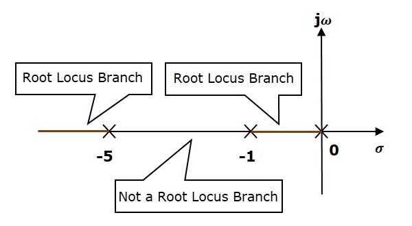
The three poles are located are shown in the above figure. The line segment between $s = 1$ and $s = 0$ is one branch of root locus on real axis. And the other branch of the root locus on the real axis is the line segment to the left of $s = 5$.
Step 2 − We will get the values of the centroid and the angle of asymptotes by using the given formulae.
Centroid $\alpha = 2$
The angle of asymptotes are $\theta = 60^0,180^0$ and $300^0$.
The centroid and three asymptotes are shown in the following figure.
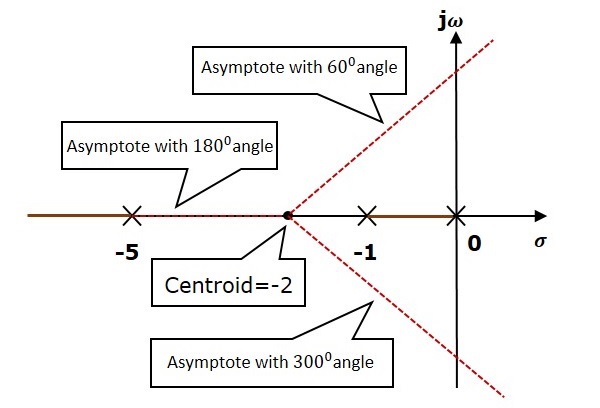
Step 3 − Since two asymptotes have the angles of $60^0$ and $300^0$, two root locus branches intersect the imaginary axis. By using the Routh array method and special case(ii), the root locus branches intersects the imaginary axis at $j\sqrt{5}$ and $j\sqrt{5}$.
There will be one break-away point on the real axis root locus branch between the poles $s = 1$ and $s = 0$. By following the procedure given for the calculation of break-away point, we will get it as $s = 0.473$.
The root locus diagram for the given control system is shown in the following figure.
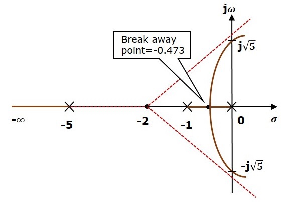
In this way, you can draw the root locus diagram of any control system and observe the movement of poles of the closed loop transfer function.
From the root locus diagrams, we can know the range of K values for different types of damping.
Effects of Adding Open Loop Poles and Zeros on Root Locus
The root locus can be shifted in s plane by adding the open loop poles and the open loop zeros.
If we include a pole in the open loop transfer function, then some of root locus branches will move towards right half of s plane. Because of this, the damping ratio $\delta$ decreases. Which implies, damped frequency $\omega_d$ increases and the time domain specifications like delay time $t_d$, rise time $t_r$ and peak time $t_p$ decrease. But, it effects the system stability.
If we include a zero in the open loop transfer function, then some of root locus branches will move towards left half of s plane. So, it will increase the control system stability. In this case, the damping ratio $\delta$ increases. Which implies, damped frequency $\omega_d$ decreases and the time domain specifications like delay time $t_d$, rise time $t_r$ and peak time $t_p$ increase.
So, based on the requirement, we can include (add) the open loop poles or zeros to the transfer function.
Frequency Response Analysis
We have already discussed time response analysis of the control systems and the time domain specifications of the second order control systems. In this chapter, let us discuss the frequency response analysis of the control systems and the frequency domain specifications of the second order control systems.
What is Frequency Response?
The response of a system can be partitioned into both the transient response and the steady state response. We can find the transient response by using Fourier integrals. The steady state response of a system for an input sinusoidal signal is known as the frequency response. In this chapter, we will focus only on the steady state response.
If a sinusoidal signal is applied as an input to a Linear Time-Invariant (LTI) system, then it produces the steady state output, which is also a sinusoidal signal. The input and output sinusoidal signals have the same frequency, but different amplitudes and phase angles.
Let the input signal be −
$$r(t)=A\sin(\omega_0t)$$
The open loop transfer function will be −
$$G(s)=G(j\omega)$$
We can represent $G(j\omega)$ in terms of magnitude and phase as shown below.
$$G(j\omega)=|G(j\omega)| \angle G(j\omega)$$
Substitute, $\omega = \omega_0$ in the above equation.
$$G(j\omega_0)=|G(j\omega_0)| \angle G(j\omega_0)$$
The output signal is
$$c(t)=A|G(j\omega_0)|\sin(\omega_0t + \angle G(j\omega_0))$$
The amplitude of the output sinusoidal signal is obtained by multiplying the amplitude of the input sinusoidal signal and the magnitude of $G(j\omega)$ at $\omega = \omega_0$.
The phase of the output sinusoidal signal is obtained by adding the phase of the input sinusoidal signal and the phase of $G(j\omega)$ at $\omega = \omega_0$.
Where,
A is the amplitude of the input sinusoidal signal.
ω0 is angular frequency of the input sinusoidal signal.
We can write, angular frequency $\omega_0$ as shown below.
$$\omega_0=2\pi f_0$$
Here, $f_0$ is the frequency of the input sinusoidal signal. Similarly, you can follow the same procedure for closed loop control system.
Frequency Domain Specifications
The frequency domain specifications are resonant peak, resonant frequency and bandwidth.
Consider the transfer function of the second order closed loop control system as,
$$T(s)=\frac{C(s)}{R(s)}=\frac{\omega_n^2}{s^2+2\delta\omega_ns+\omega_n^2}$$
Substitute, $s = j\omega$ in the above equation.
$$T(j\omega)=\frac{\omega_n^2}{(j\omega)^2+2\delta\omega_n(j\omega)+\omega_n^2}$$
$$\Rightarrow T(j\omega)=\frac{\omega_n^2}{-\omega^2+2j\delta\omega\omega_n+\omega_n^2}=\frac{\omega_n^2}{\omega_n^2\left ( 1-\frac{\omega^2}{\omega_n^2}+\frac{2j\delta\omega}{\omega_n} \right )}$$
$$\Rightarrow T(j\omega)=\frac{1}{\left ( 1-\frac{\omega^2}{\omega_n^2} \right )+j\left ( \frac{2\delta\omega}{\omega_n} \right )}$$
Let, $\frac{\omega}{\omega_n}=u$ Substitute this value in the above equation.
$$T(j\omega)=\frac{1}{(1-u^2)+j(2\delta u)}$$
Magnitude of $T(j\omega)$ is -
$$M=|T(j\omega)|=\frac{1}{\sqrt {(1-u^2)^2+(2\delta u)^2}}$$
Phase of $T(j\omega)$ is -
$$\angle T(j\omega)=-tan^{-1}\left( \frac{2\delta u}{1-u^2} \right )$$
Resonant Frequency
It is the frequency at which the magnitude of the frequency response has peak value for the first time. It is denoted by $\omega_r$. At $\omega = \omega_r$, the first derivate of the magnitude of $T(j\omega)$ is zero.
Differentiate $M$ with respect to $u$.
$$\frac{\text{d}M}{\text{d}u}=-\frac{1}{2}\left [ (1-u^2)^2+(2\delta u)^2 \right ]^{\frac{-3}{2}} \left [2(1-u^2)(-2u)+2(2\delta u)(2\delta) \right ]$$
$$\Rightarrow \frac{\text{d}M}{\text{d}u}=-\frac{1}{2}\left [ (1-u^2)^2+(2\delta u)^2 \right ]^{\frac{-3}{2}} \left [4u(u^2-1 +2\delta^2) \right ]$$
Substitute, $u=u_r$ and $\frac{\text{d}M}{\text{d}u}==0$ in the above equation.
$$0=-\frac{1}{2}\left [ (1-u_r^2)^2+(2\delta u_r)^2 \right ]^{-\frac{3}{2}}\left [ 4u_r(u_r^2-1 +2\delta^2) \right ]$$
$$\Rightarrow 4u_r(u_r^2-1 +2\delta^2)=0$$
$$\Rightarrow u_r^2-1+2\delta^2=0$$
$$\Rightarrow u_r^2=1-2\delta^2$$
$$\Rightarrow u_r=\sqrt{1-2\delta^2}$$
Substitute, $u_r=\frac{\omega_r}{\omega_n}$ in the above equation.
$$\frac{\omega_r}{\omega_n}=\sqrt{1-2\delta^2}$$
$$\Rightarrow \omega_r=\omega_n \sqrt{1-2\delta^2}$$
Resonant Peak
It is the peak (maximum) value of the magnitude of $T(j\omega)$. It is denoted by $M_r$.
At $u = u_r$, the Magnitude of $T(j\omega)$ is -
$$M_r=\frac{1}{\sqrt{(1-u_r^2)^2+(2\delta u_r)^2}}$$
Substitute, $u_r = \sqrt{1 2\delta^2}$ and $1 u_r^2 = 2\delta^2$ in the above equation.
$$M_r=\frac{1}{\sqrt{(2\delta^2)^2+(2\delta \sqrt{1-2\delta^2})^2}}$$
$$\Rightarrow M_r=\frac{1}{2\delta \sqrt {1-\delta^2}}$$
Resonant peak in frequency response corresponds to the peak overshoot in the time domain transient response for certain values of damping ratio $\delta$. So, the resonant peak and peak overshoot are correlated to each other.
Bandwidth
It is the range of frequencies over which, the magnitude of $T(j\omega)$ drops to 70.7% from its zero frequency value.
At $\omega = 0$, the value of $u$ will be zero.
Substitute, $u = 0$ in M.
$$M=\frac{1}{\sqrt {(1-0^2)^2+(2\delta(0))^2}}=1$$
Therefore, the magnitude of $T(j\omega)$ is one at $\omega = 0$.
At 3-dB frequency, the magnitude of $T(j\omega)$ will be 70.7% of magnitude of $T(j\omega)$ at $\omega = 0$.
i.e., at $\omega = \omega_B, M = 0.707(1) = \frac{1}{\sqrt{2}}$
$$\Rightarrow M=\frac{1}{\sqrt{2}}=\frac{1}{\sqrt{(1-u_b^2)^2+(2\delta u_b)^2}}$$
$$\Rightarrow 2=(1-u_b^2)^2+(2\delta)^2 u_b^2$$
Let, $u_b^2=x$
$$\Rightarrow 2=(1-x)^2+(2\delta)^2 x$$
$$\Rightarrow x^2+(4\delta^2-2)x-1=0$$
$$\Rightarrow x=\frac{-(4\delta^2 -2)\pm \sqrt{(4\delta^2-2)^2+4}}{2}$$
Consider only the positive value of x.
$$x=1-2\delta^2+\sqrt {(2\delta^2-1)^2+1}$$
$$\Rightarrow x=1-2\delta^2+\sqrt {(2-4\delta^2+4\delta^4)}$$
Substitute, $x=u_b^2=\frac{\omega_b^2}{\omega_n^2}$
$$\frac{\omega_b^2}{\omega_n^2}=1-2\delta^2+\sqrt {(2-4\delta^2+4\delta^4)}$$
$$\Rightarrow \omega_b=\omega_n \sqrt {1-2\delta^2+\sqrt {(2-4\delta^2+4\delta^4)}}$$
Bandwidth $\omega_b$ in the frequency response is inversely proportional to the rise time $t_r$ in the time domain transient response.
Control Systems - Bode Plots
The Bode plot or the Bode diagram consists of two plots −
- Magnitude plot
- Phase plot
In both the plots, x-axis represents angular frequency (logarithmic scale). Whereas, yaxis represents the magnitude (linear scale) of open loop transfer function in the magnitude plot and the phase angle (linear scale) of the open loop transfer function in the phase plot.
The magnitude of the open loop transfer function in dB is -
$$M=20\: \log|G(j\omega)H(j\omega)|$$
The phase angle of the open loop transfer function in degrees is -
$$\phi=\angle G(j\omega)H(j\omega)$$
Note − The base of logarithm is 10.
Basic of Bode Plots
The following table shows the slope, magnitude and the phase angle values of the terms present in the open loop transfer function. This data is useful while drawing the Bode plots.
| Type of term | G(jω)H(jω) | Slope(dB/dec) | Magnitude (dB) | Phase angle(degrees) |
|---|---|---|---|---|
Constant |
$K$ |
$0$ |
$20 \log K$ |
$0$ |
Zero at origin |
$j\omega$ |
$20$ |
$20 \log \omega$ |
$90$ |
n zeros at origin |
$(j\omega)^n$ |
$20\: n$ |
$20\: n \log \omega$ |
$90\: n$ |
Pole at origin |
$\frac{1}{j\omega}$ |
$-20$ |
$-20 \log \omega$ |
$-90 \: or \: 270$ |
n poles at origin |
$\frac{1}{(j\omega)^n}$ |
$-20\: n$ |
$-20 \: n \log \omega$ |
$-90 \: n \: or \: 270 \: n$ |
Simple zero |
$1+j\omega r$ |
$20$ |
$0\: for\: \omega < \frac{1}{r}$ $20\: \log \omega r\: for \: \omega > \frac{1}{r}$ |
$0 \: for \: \omega < \frac{1}{r}$ $90 \: for \: \omega > \frac{1}{r}$ |
Simple pole |
$\frac{1}{1+j\omega r}$ |
$-20$ |
$0\: for\: \omega < \frac{1}{r}$ $-20\: \log \omega r\: for\: \omega > \frac{1}{r}$ |
$0 \: for \: \omega < \frac{1}{r}$ $-90\: or \: 270 \: for\: \omega > \frac{1}{r}$ |
Second order derivative term |
$\omega_n^2\left ( 1-\frac{\omega^2}{\omega_n^2}+\frac{2j\delta\omega}{\omega_n} \right )$ |
$40$ |
$40\: \log\: \omega_n\: for \: \omega < \omega_n$ $20\: \log\:(2\delta\omega_n^2)\: for \: \omega=\omega_n$ $40 \: \log \: \omega\:for \:\omega > \omega_n$ |
$0 \: for \: \omega < \omega_n$ $90 \: for \: \omega = \omega_n$ $180 \: for \: \omega > \omega_n$ |
Second order integral term |
$\frac{1}{\omega_n^2\left ( 1-\frac{\omega^2}{\omega_n^2}+\frac{2j\delta\omega}{\omega_n} \right )}$ |
$-40$ |
$-40\: \log\: \omega_n\: for \: \omega < \omega_n$ $-20\: \log\:(2\delta\omega_n^2)\: for \: \omega=\omega_n$ $-40 \: \log \: \omega\:for \:\omega > \omega_n$ |
$-0 \: for \: \omega < \omega_n$ $-90 \: for \: \omega = \omega_n$ $-180 \: for \: \omega > \omega_n$ |
Consider the open loop transfer function $G(s)H(s) = K$.
Magnitude $M = 20\: \log K$ dB
Phase angle $\phi = 0$ degrees
If $K = 1$, then magnitude is 0 dB.
If $K > 1$, then magnitude will be positive.
If $K < 1$, then magnitude will be negative.
The following figure shows the corresponding Bode plot.
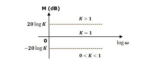
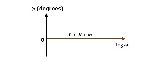
The magnitude plot is a horizontal line, which is independent of frequency. The 0 dB line itself is the magnitude plot when the value of K is one. For the positive values of K, the horizontal line will shift $20 \:\log K$ dB above the 0 dB line. For the negative values of K, the horizontal line will shift $20\: \log K$ dB below the 0 dB line. The Zero degrees line itself is the phase plot for all the positive values of K.
Consider the open loop transfer function $G(s)H(s) = s$.
Magnitude $M = 20 \log \omega$ dB
Phase angle $\phi = 90^0$
At $\omega = 0.1$ rad/sec, the magnitude is -20 dB.
At $\omega = 1$ rad/sec, the magnitude is 0 dB.
At $\omega = 10$ rad/sec, the magnitude is 20 dB.
The following figure shows the corresponding Bode plot.
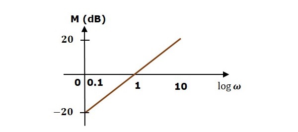
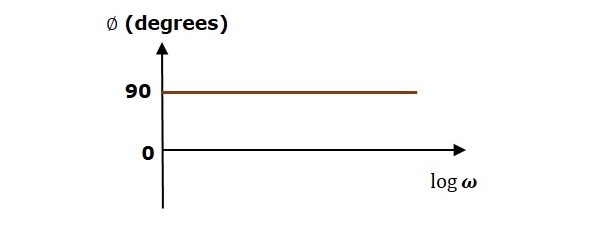
The magnitude plot is a line, which is having a slope of 20 dB/dec. This line started at $\omega = 0.1$ rad/sec having a magnitude of -20 dB and it continues on the same slope. It is touching 0 dB line at $\omega = 1$ rad/sec. In this case, the phase plot is 900 line.
Consider the open loop transfer function $G(s)H(s) = 1 + s\tau$.
Magnitude $M = 20\: log \sqrt{1 + \omega^2\tau^2}$ dB
Phase angle $\phi = \tan^{-1}\omega\tau$ degrees
For $ < \frac{1}{\tau}$ , the magnitude is 0 dB and phase angle is 0 degrees.
For $\omega > \frac{1}{\tau}$ , the magnitude is $20\: \log \omega\tau$ dB and phase angle is 900.
The following figure shows the corresponding Bode plot.
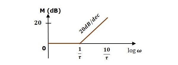
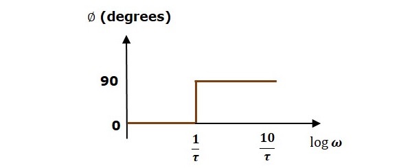
The magnitude plot is having magnitude of 0 dB upto $\omega=\frac{1}{\tau}$ rad/sec. From $\omega = \frac{1}{\tau}$ rad/sec, it is having a slope of 20 dB/dec. In this case, the phase plot is having phase angle of 0 degrees up to $\omega = \frac{1}{\tau}$ rad/sec and from here, it is having phase angle of 900. This Bode plot is called the asymptotic Bode plot.
As the magnitude and the phase plots are represented with straight lines, the Exact Bode plots resemble the asymptotic Bode plots. The only difference is that the Exact Bode plots will have simple curves instead of straight lines.
Similarly, you can draw the Bode plots for other terms of the open loop transfer function which are given in the table.
Control Systems - Construction of Bode Plots
In this chapter, let us understand in detail how to construct (draw) Bode plots.
Rules for Construction of Bode Plots
Follow these rules while constructing a Bode plot.
Represent the open loop transfer function in the standard time constant form.
Substitute, $s=j\omega$ in the above equation.
Find the corner frequencies and arrange them in ascending order.
Consider the starting frequency of the Bode plot as 1/10th of the minimum corner frequency or 0.1 rad/sec whichever is smaller value and draw the Bode plot upto 10 times maximum corner frequency.
Draw the magnitude plots for each term and combine these plots properly.
Draw the phase plots for each term and combine these plots properly.
Note − The corner frequency is the frequency at which there is a change in the slope of the magnitude plot.
Example
Consider the open loop transfer function of a closed loop control system
$$G(s)H(s)=\frac{10s}{(s+2)(s+5)}$$
Let us convert this open loop transfer function into standard time constant form.
$$G(s)H(s)=\frac{10s}{2\left( \frac{s}{2}+1 \right )5 \left( \frac{s}{5}+1 \right )}$$
$$\Rightarrow G(s)H(s)=\frac{s}{\left( 1+\frac{s}{2} \right )\left( 1+\frac{s}{5} \right )}$$
So, we can draw the Bode plot in semi log sheet using the rules mentioned earlier.
Stability Analysis using Bode Plots
From the Bode plots, we can say whether the control system is stable, marginally stable or unstable based on the values of these parameters.
- Gain cross over frequency and phase cross over frequency
- Gain margin and phase margin
Phase Cross over Frequency
The frequency at which the phase plot is having the phase of -1800 is known as phase cross over frequency. It is denoted by $\omega_{pc}$. The unit of phase cross over frequency is rad/sec.
Gain Cross over Frequency
The frequency at which the magnitude plot is having the magnitude of zero dB is known as gain cross over frequency. It is denoted by $\omega_{gc}$. The unit of gain cross over frequency is rad/sec.
The stability of the control system based on the relation between the phase cross over frequency and the gain cross over frequency is listed below.
If the phase cross over frequency $\omega_{pc}$ is greater than the gain cross over frequency $\omega_{gc}$, then the control system is stable.
If the phase cross over frequency $\omega_{pc}$ is equal to the gain cross over frequency $\omega_{gc}$, then the control system is marginally stable.
If the phase cross over frequency $\omega_{pc}$ is less than the gain cross over frequency $\omega_{gc}$, then the control system is unstable.
Gain Margin
Gain margin $GM$ is equal to negative of the magnitude in dB at phase cross over frequency.
$$GM=20\log\left( \frac{1}{M_{pc}}\right )=20logM_{pc}$$
Where, $M_{pc}$ is the magnitude at phase cross over frequency. The unit of gain margin (GM) is dB.
Phase Margin
The formula for phase margin $PM$ is
$$PM=180^0+\phi_{gc}$$
Where, $\phi_{gc}$ is the phase angle at gain cross over frequency. The unit of phase margin is degrees.
The stability of the control system based on the relation between gain margin and phase margin is listed below.
If both the gain margin $GM$ and the phase margin $PM$ are positive, then the control system is stable.
If both the gain margin $GM$ and the phase margin $PM$ are equal to zero, then the control system is marginally stable.
If the gain margin $GM$ and / or the phase margin $PM$ are/is negative, then the control system is unstable.
Control Systems - Polar Plots
In the previous chapters, we discussed the Bode plots. There, we have two separate plots for both magnitude and phase as the function of frequency. Let us now discuss about polar plots. Polar plot is a plot which can be drawn between magnitude and phase. Here, the magnitudes are represented by normal values only.
The polar form of $G(j\omega)H(j\omega)$ is
$$G(j\omega)H(j\omega)=|G(j\omega)H(j\omega)| \angle G(j\omega)H(j\omega)$$
The Polar plot is a plot, which can be drawn between the magnitude and the phase angle of $G(j\omega)H(j\omega)$ by varying $\omega$ from zero to ∞. The polar graph sheet is shown in the following figure.
This graph sheet consists of concentric circles and radial lines. The concentric circles and the radial lines represent the magnitudes and phase angles respectively. These angles are represented by positive values in anti-clock wise direction. Similarly, we can represent angles with negative values in clockwise direction. For example, the angle 2700 in anti-clock wise direction is equal to the angle 900 in clockwise direction.
Rules for Drawing Polar Plots
Follow these rules for plotting the polar plots.
Substitute, $s = j\omega$ in the open loop transfer function.
Write the expressions for magnitude and the phase of $G(j\omega)H(j\omega)$.
Find the starting magnitude and the phase of $G(j\omega)H(j\omega)$ by substituting $\omega = 0$. So, the polar plot starts with this magnitude and the phase angle.
Find the ending magnitude and the phase of $G(j\omega)H(j\omega)$ by substituting $\omega = \infty$. So, the polar plot ends with this magnitude and the phase angle.
Check whether the polar plot intersects the real axis, by making the imaginary term of $G(j\omega)H(j\omega)$ equal to zero and find the value(s) of $\omega$.
Check whether the polar plot intersects the imaginary axis, by making real term of $G(j\omega)H(j\omega)$ equal to zero and find the value(s) of $\omega$.
For drawing polar plot more clearly, find the magnitude and phase of $G(j\omega)H(j\omega)$ by considering the other value(s) of $\omega$.
Example
Consider the open loop transfer function of a closed loop control system.
$$G(s)H(s)=\frac{5}{s(s+1)(s+2)}$$
Let us draw the polar plot for this control system using the above rules.
Step 1 − Substitute, $s = j\omega$ in the open loop transfer function.
$$G(j\omega)H(j\omega)=\frac{5}{j\omega(j\omega+1)(j\omega+2)}$$
The magnitude of the open loop transfer function is
$$M=\frac{5}{\omega(\sqrt{\omega^2+1})(\sqrt{\omega^2+4})}$$
The phase angle of the open loop transfer function is
$$\phi=-90^0-\tan^{-1}\omega-\tan^{-1}\frac{\omega}{2}$$
Step 2 − The following table shows the magnitude and the phase angle of the open loop transfer function at $\omega = 0$ rad/sec and $\omega = \infty$ rad/sec.
| Frequency (rad/sec) | Magnitude | Phase angle(degrees) |
|---|---|---|
| 0 | ∞ | -90 or 270 |
| ∞ | 0 | -270 or 90 |
So, the polar plot starts at (∞,900) and ends at (0,2700). The first and the second terms within the brackets indicate the magnitude and phase angle respectively.
Step 3 − Based on the starting and the ending polar co-ordinates, this polar plot will intersect the negative real axis. The phase angle corresponding to the negative real axis is 1800 or 1800. So, by equating the phase angle of the open loop transfer function to either 1800 or 1800, we will get the $\omega$ value as $\sqrt{2}$.
By substituting $\omega = \sqrt{2}$ in the magnitude of the open loop transfer function, we will get $M = 0.83$. Therefore, the polar plot intersects the negative real axis when $\omega = \sqrt{2}$ and the polar coordinate is (0.83,1800).
So, we can draw the polar plot with the above information on the polar graph sheet.
Control Systems - Nyquist Plots
Nyquist plots are the continuation of polar plots for finding the stability of the closed loop control systems by varying ω from ∞ to ∞. That means, Nyquist plots are used to draw the complete frequency response of the open loop transfer function.
Nyquist Stability Criterion
The Nyquist stability criterion works on the principle of argument. It states that if there are P poles and Z zeros are enclosed by the s plane closed path, then the corresponding $G(s)H(s)$ plane must encircle the origin $P Z$ times. So, we can write the number of encirclements N as,
$$N=P-Z$$
If the enclosed s plane closed path contains only poles, then the direction of the encirclement in the $G(s)H(s)$ plane will be opposite to the direction of the enclosed closed path in the s plane.
If the enclosed s plane closed path contains only zeros, then the direction of the encirclement in the $G(s)H(s)$ plane will be in the same direction as that of the enclosed closed path in the s plane.
Let us now apply the principle of argument to the entire right half of the s plane by selecting it as a closed path. This selected path is called the Nyquist contour.
We know that the closed loop control system is stable if all the poles of the closed loop transfer function are in the left half of the s plane. So, the poles of the closed loop transfer function are nothing but the roots of the characteristic equation. As the order of the characteristic equation increases, it is difficult to find the roots. So, let us correlate these roots of the characteristic equation as follows.
The Poles of the characteristic equation are same as that of the poles of the open loop transfer function.
The zeros of the characteristic equation are same as that of the poles of the closed loop transfer function.
We know that the open loop control system is stable if there is no open loop pole in the the right half of the s plane.
i.e.,$P=0 \Rightarrow N=-Z$
We know that the closed loop control system is stable if there is no closed loop pole in the right half of the s plane.
i.e.,$Z=0 \Rightarrow N=P$
Nyquist stability criterion states the number of encirclements about the critical point (1+j0) must be equal to the poles of characteristic equation, which is nothing but the poles of the open loop transfer function in the right half of the s plane. The shift in origin to (1+j0) gives the characteristic equation plane.
Rules for Drawing Nyquist Plots
Follow these rules for plotting the Nyquist plots.
Locate the poles and zeros of open loop transfer function $G(s)H(s)$ in s plane.
Draw the polar plot by varying $\omega$ from zero to infinity. If pole or zero present at s = 0, then varying $\omega$ from 0+ to infinity for drawing polar plot.
Draw the mirror image of above polar plot for values of $\omega$ ranging from ∞ to zero (0 if any pole or zero present at s=0).
The number of infinite radius half circles will be equal to the number of poles or zeros at origin. The infinite radius half circle will start at the point where the mirror image of the polar plot ends. And this infinite radius half circle will end at the point where the polar plot starts.
After drawing the Nyquist plot, we can find the stability of the closed loop control system using the Nyquist stability criterion. If the critical point (-1+j0) lies outside the encirclement, then the closed loop control system is absolutely stable.
Stability Analysis using Nyquist Plots
From the Nyquist plots, we can identify whether the control system is stable, marginally stable or unstable based on the values of these parameters.
- Gain cross over frequency and phase cross over frequency
- Gain margin and phase margin
Phase Cross over Frequency
The frequency at which the Nyquist plot intersects the negative real axis (phase angle is 1800) is known as the phase cross over frequency. It is denoted by $\omega_{pc}$.
Gain Cross over Frequency
The frequency at which the Nyquist plot is having the magnitude of one is known as the gain cross over frequency. It is denoted by $\omega_{gc}$.
The stability of the control system based on the relation between phase cross over frequency and gain cross over frequency is listed below.
If the phase cross over frequency $\omega_{pc}$ is greater than the gain cross over frequency $\omega_{gc}$, then the control system is stable.
If the phase cross over frequency $\omega_{pc}$ is equal to the gain cross over frequency $\omega_{gc}$, then the control system is marginally stable.
If phase cross over frequency $\omega_{pc}$ is less than gain cross over frequency $\omega_{gc}$, then the control system is unstable.
Gain Margin
The gain margin $GM$ is equal to the reciprocal of the magnitude of the Nyquist plot at the phase cross over frequency.
$$GM=\frac{1}{M_{pc}}$$
Where, $M_{pc}$ is the magnitude in normal scale at the phase cross over frequency.
Phase Margin
The phase margin $PM$ is equal to the sum of 1800 and the phase angle at the gain cross over frequency.
$$PM=180^0+\phi_{gc}$$
Where, $\phi_{gc}$ is the phase angle at the gain cross over frequency.
The stability of the control system based on the relation between the gain margin and the phase margin is listed below.
If the gain margin $GM$ is greater than one and the phase margin $PM$ is positive, then the control system is stable.
If the gain margin $GM$ is equal to one and the phase margin $PM$ is zero degrees, then the control system is marginally stable.
If the gain margin $GM$ is less than one and / or the phase margin $PM$ is negative, then the control system is unstable.
Control Systems - Compensators
There are three types of compensators lag, lead and lag-lead compensators. These are most commonly used.
Lag Compensator
The Lag Compensator is an electrical network which produces a sinusoidal output having the phase lag when a sinusoidal input is applied. The lag compensator circuit in the s domain is shown in the following figure.
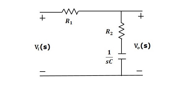
Here, the capacitor is in series with the resistor $R_2$ and the output is measured across this combination.
The transfer function of this lag compensator is -
$$\frac{V_o(s)}{V_i(s)}=\frac{1}{\alpha} \left( \frac{s+\frac{1}{\tau}}{s+\frac{1}{\alpha\tau}} \right )$$
Where,
$$\tau=R_2C$$
$$\alpha=\frac{R_1+R_2}{R_2}$$
From the above equation, $\alpha$ is always greater than one.
From the transfer function, we can conclude that the lag compensator has one pole at $s = \frac{1}{\alpha \tau}$ and one zero at $s = \frac{1}{\tau}$ . This means, the pole will be nearer to origin in the pole-zero configuration of the lag compensator.
Substitute, $s = j\omega$ in the transfer function.
$$\frac{V_o(j\omega)}{V_i(j\omega)}=\frac{1}{\alpha}\left( \frac{j\omega+\frac{1}{\tau}}{j\omega+\frac{1}{\alpha\tau}}\right )$$
Phase angle $\phi = \tan^{1} \omega\tau tan^{1} \alpha\omega\tau$
We know that, the phase of the output sinusoidal signal is equal to the sum of the phase angles of input sinusoidal signal and the transfer function.
So, in order to produce the phase lag at the output of this compensator, the phase angle of the transfer function should be negative. This will happen when $\alpha > 1$.
Lead Compensator
The lead compensator is an electrical network which produces a sinusoidal output having phase lead when a sinusoidal input is applied. The lead compensator circuit in the s domain is shown in the following figure.
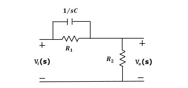
Here, the capacitor is parallel to the resistor $R_1$ and the output is measured across resistor $R_2.
The transfer function of this lead compensator is -
$$\frac{V_o(s)}{V_i(s)}=\beta \left( \frac{s\tau+1}{\beta s\tau+1} \right )$$
Where,
$$\tau=R_1C$$
$$\beta=\frac{R_2}{R_1+R_2}$$
From the transfer function, we can conclude that the lead compensator has pole at $s = \frac{1}{\beta}$ and zero at $s = \frac{1}{\beta\tau}$.
Substitute, $s = j\omega$ in the transfer function.
$$\frac{V_o(j\omega)}{V_i(j\omega)}=\beta \left( \frac{j\omega\tau+1}{\beta j \omega\tau+1} \right )$$
Phase angle $\phi = tan^{1}\omega\tau tan^{1}\beta\omega\tau$
We know that, the phase of the output sinusoidal signal is equal to the sum of the phase angles of input sinusoidal signal and the transfer function.
So, in order to produce the phase lead at the output of this compensator, the phase angle of the transfer function should be positive. This will happen when $0 < \beta < 1$. Therefore, zero will be nearer to origin in pole-zero configuration of the lead compensator.
Lag-Lead Compensator
Lag-Lead compensator is an electrical network which produces phase lag at one frequency region and phase lead at other frequency region. It is a combination of both the lag and the lead compensators. The lag-lead compensator circuit in the s domain is shown in the following figure.
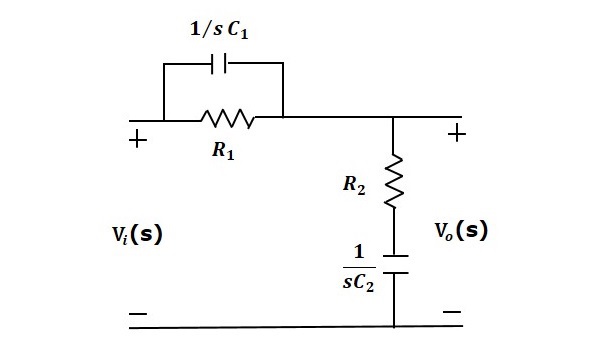
This circuit looks like both the compensators are cascaded. So, the transfer function of this circuit will be the product of transfer functions of the lead and the lag compensators.
$$\frac{V_o(s)}{V_i(s)}=\beta \left( \frac{s\tau_1+1}{\beta s \tau_1+1} \right )\frac{1}{\alpha} \left ( \frac{s+\frac{1}{\tau_2}}{s+\frac{1}{\alpha\tau_2}} \right )$$
We know $\alpha\beta=1$.
$$\Rightarrow \frac{V_o(s)}{V_i(s)}=\left ( \frac{s+\frac{1}{\tau_1}}{s+\frac{1}{\beta\tau_1}} \right )\left ( \frac{s+\frac{1}{\tau_2}}{s+\frac{1}{\alpha\tau_2}} \right )$$
Where,
$$\tau_1=R_1C_1$$
$$\tau_2=R_2C_2$$
Control Systems - Controllers
The various types of controllers are used to improve the performance of control systems. In this chapter, we will discuss the basic controllers such as the proportional, the derivative and the integral controllers.
Proportional Controller
The proportional controller produces an output, which is proportional to error signal.
$$u(t) \propto e(t) $$
$$\Rightarrow u(t)=K_P e(t)$$
Apply Laplace transform on both the sides -
$$U(s)=K_P E(s)$$
$$\frac{U(s)}{E(s)}=K_P$$
Therefore, the transfer function of the proportional controller is $K_P$.
Where,
U(s) is the Laplace transform of the actuating signal u(t)
E(s) is the Laplace transform of the error signal e(t)
KP is the proportionality constant
The block diagram of the unity negative feedback closed loop control system along with the proportional controller is shown in the following figure.
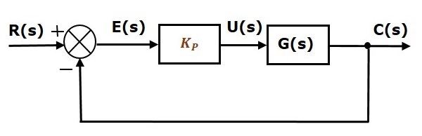
The proportional controller is used to change the transient response as per the requirement.
Derivative Controller
The derivative controller produces an output, which is derivative of the error signal.
$$u(t)=K_D \frac{\text{d}e(t)}{\text{d}t}$$
Apply Laplace transform on both sides.
$$U(s)=K_D sE(s)$$
$$\frac{U(s)}{E(s)}=K_D s$$
Therefore, the transfer function of the derivative controller is $K_D s$.
Where, $K_D$ is the derivative constant.
The block diagram of the unity negative feedback closed loop control system along with the derivative controller is shown in the following figure.
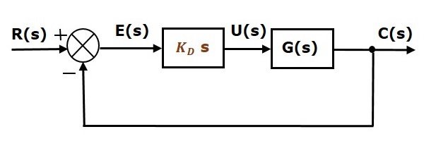
The derivative controller is used to make the unstable control system into a stable one.
Integral Controller
The integral controller produces an output, which is integral of the error signal.
$$u(t)=K_I \int e(t) dt$$
Apply Laplace transform on both the sides -
$$U(s)=\frac{K_I E(s)}{s}$$
$$\frac{U(s)}{E(s)}=\frac{K_I}{s}$$
Therefore, the transfer function of the integral controller is $\frac{K_I}{s}$.
Where, $K_I$ is the integral constant.
The block diagram of the unity negative feedback closed loop control system along with the integral controller is shown in the following figure.
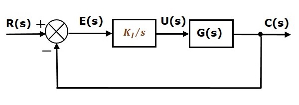
The integral controller is used to decrease the steady state error.
Let us now discuss about the combination of basic controllers.
Proportional Derivative (PD) Controller
The proportional derivative controller produces an output, which is the combination of the outputs of proportional and derivative controllers.
$$u(t)=K_P e(t)+K_D \frac{\text{d}e(t)}{\text{d}t}$$
Apply Laplace transform on both sides -
$$U(s)=(K_P+K_D s)E(s)$$
$$\frac{U(s)}{E(s)}=K_P+K_D s$$
Therefore, the transfer function of the proportional derivative controller is $K_P + K_D s$.
The block diagram of the unity negative feedback closed loop control system along with the proportional derivative controller is shown in the following figure.
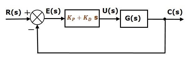
The proportional derivative controller is used to improve the stability of control system without affecting the steady state error.
Proportional Integral (PI) Controller
The proportional integral controller produces an output, which is the combination of outputs of the proportional and integral controllers.
$$u(t)=K_P e(t)+K_I \int e(t) dt$$
Apply Laplace transform on both sides -
$$U(s)=\left(K_P+\frac{K_I}{s} \right )E(s)$$
$$\frac{U(s)}{E(s)}=K_P+\frac{K_I}{s}$$
Therefore, the transfer function of proportional integral controller is $K_P + \frac{K_I} {s}$.
The block diagram of the unity negative feedback closed loop control system along with the proportional integral controller is shown in the following figure.
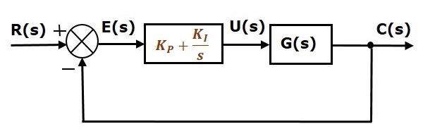
The proportional integral controller is used to decrease the steady state error without affecting the stability of the control system.
Proportional Integral Derivative (PID) Controller
The proportional integral derivative controller produces an output, which is the combination of the outputs of proportional, integral and derivative controllers.
$$u(t)=K_P e(t)+K_I \int e(t) dt+K_D \frac{\text{d}e(t)}{\text{d}t}$$
Apply Laplace transform on both sides -
$$U(s)=\left(K_P+\frac{K_I}{s}+K_D s \right )E(s)$$
$$\frac{U(s)}{E(s)}=K_P+\frac{K_I}{s}+K_D s$$
Therefore, the transfer function of the proportional integral derivative controller is $K_P + \frac{K_I} {s} + K_D s$.
The block diagram of the unity negative feedback closed loop control system along with the proportional integral derivative controller is shown in the following figure.
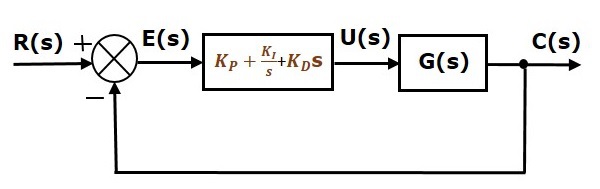
The proportional integral derivative controller is used to improve the stability of the control system and to decrease steady state error.
Control Systems - State Space Model
The state space model of Linear Time-Invariant (LTI) system can be represented as,
$$\dot{X}=AX+BU$$
$$Y=CX+DU$$
The first and the second equations are known as state equation and output equation respectively.
Where,
X and $\dot{X}$ are the state vector and the differential state vector respectively.
U and Y are input vector and output vector respectively.
A is the system matrix.
B and C are the input and the output matrices.
D is the feed-forward matrix.
Basic Concepts of State Space Model
The following basic terminology involved in this chapter.
State
It is a group of variables, which summarizes the history of the system in order to predict the future values (outputs).
State Variable
The number of the state variables required is equal to the number of the storage elements present in the system.
Examples − current flowing through inductor, voltage across capacitor
State Vector
It is a vector, which contains the state variables as elements.
In the earlier chapters, we have discussed two mathematical models of the control systems. Those are the differential equation model and the transfer function model. The state space model can be obtained from any one of these two mathematical models. Let us now discuss these two methods one by one.
State Space Model from Differential Equation
Consider the following series of the RLC circuit. It is having an input voltage, $v_i(t)$ and the current flowing through the circuit is $i(t)$.
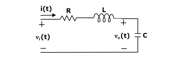
There are two storage elements (inductor and capacitor) in this circuit. So, the number of the state variables is equal to two and these state variables are the current flowing through the inductor, $i(t)$ and the voltage across capacitor, $v_c(t)$.
From the circuit, the output voltage, $v_0(t)$ is equal to the voltage across capacitor, $v_c(t)$.
$$v_0(t)=v_c(t)$$
Apply KVL around the loop.
$$v_i(t)=Ri(t)+L\frac{\text{d}i(t)}{\text{d}t}+v_c(t)$$
$$\Rightarrow \frac{\text{d}i(t)}{\text{d}t}=-\frac{Ri(t)}{L}-\frac{v_c(t)}{L}+\frac{v_i(t)}{L}$$
The voltage across the capacitor is -
$$v_c(t)=\frac{1}{C} \int i(t) dt$$
Differentiate the above equation with respect to time.
$$\frac{\text{d}v_c(t)}{\text{d}t}=\frac{i(t)}{C}$$
State vector, $X=\begin{bmatrix}i(t) \\v_c(t) \end{bmatrix}$
Differential state vector, $\dot{X}=\begin{bmatrix}\frac{\text{d}i(t)}{\text{d}t} \\\frac{\text{d}v_c(t)}{\text{d}t} \end{bmatrix}$
We can arrange the differential equations and output equation into the standard form of state space model as,
$$\dot{X}=\begin{bmatrix}\frac{\text{d}i(t)}{\text{d}t} \\\frac{\text{d}v_c(t)}{\text{d}t} \end{bmatrix}=\begin{bmatrix}-\frac{R}{L} & -\frac{1}{L} \\\frac{1}{C} & 0 \end{bmatrix}\begin{bmatrix}i(t) \\v_c(t) \end{bmatrix}+\begin{bmatrix}\frac{1}{L} \\0 \end{bmatrix}\begin{bmatrix}v_i(t) \end{bmatrix}$$
$$Y=\begin{bmatrix}0 & 1 \end{bmatrix}\begin{bmatrix}i(t) \\v_c(t) \end{bmatrix}$$
Where,
$$A=\begin{bmatrix}-\frac{R}{L} & -\frac{1}{L} \\\frac{1}{C} & 0 \end{bmatrix}, \: B=\begin{bmatrix}\frac{1}{L} \\0 \end{bmatrix}, \: C=\begin{bmatrix}0 & 1 \end{bmatrix} \: and \: D=\begin{bmatrix}0 \end{bmatrix}$$
State Space Model from Transfer Function
Consider the two types of transfer functions based on the type of terms present in the numerator.
- Transfer function having constant term in Numerator.
- Transfer function having polynomial function of s in Numerator.
Transfer function having constant term in Numerator
Consider the following transfer function of a system
$$\frac{Y(s)}{U(s)}=\frac{b_0}{s^n+a_{n-1}s^{n-1}+...+a_1s+a_0}$$
Rearrange, the above equation as
$$(s^n+a_{n-1}s^{n-1}+...+a_0)Y(s)=b_0 U(s)$$
Apply inverse Laplace transform on both sides.
$$\frac{\text{d}^ny(t)}{\text{d}t^n}+a_{n-1}\frac{\text{d}^{n-1}y(t)}{\text{d}t^{n-1}}+...+a_1\frac{\text{d}y(t)}{\text{d}t}+a_0y(t)=b_0 u(t)$$
Let
$$y(t)=x_1$$
$$\frac{\text{d}y(t)}{\text{d}t}=x_2=\dot{x}_1$$
$$\frac{\text{d}^2y(t)}{\text{d}t^2}=x_3=\dot{x}_2$$
$$.$$
$$.$$
$$.$$
$$\frac{\text{d}^{n-1}y(t)}{\text{d}t^{n-1}}=x_n=\dot{x}_{n-1}$$
$$\frac{\text{d}^ny(t)}{\text{d}t^n}=\dot{x}_n$$
and $u(t)=u$
Then,
$$\dot{x}_n+a_{n-1}x_n+...+a_1x_2+a_0x_1=b_0 u$$
From the above equation, we can write the following state equation.
$$\dot{x}_n=-a_0x_1-a_1x_2-...-a_{n-1}x_n+b_0 u$$
The output equation is -
$$y(t)=y=x_1$$
The state space model is -
$\dot{X}=\begin{bmatrix}\dot{x}_1 \\\dot{x}_2 \\\vdots \\\dot{x}_{n-1} \\\dot{x}_n \end{bmatrix}$
$$=\begin{bmatrix}0 & 1 & 0 & \dotso & 0 & 0 \\0 & 0 & 1 & \dotso & 0 & 0 \\\vdots & \vdots & \vdots & \dotso & \vdots & \vdots \\ 0 & 0 & 0 & \dotso & 0 & 1 \\-a_0 & -a_1 & -a_2 & \dotso & -a_{n-2} & -a_{n-1} \end{bmatrix} \begin{bmatrix}x_1 \\x_2 \\\vdots \\x_{n-1} \\x_n \end{bmatrix}+\begin{bmatrix}0 \\0 \\\vdots \\0 \\b_0 \end{bmatrix}\begin{bmatrix}u \end{bmatrix}$$
$$Y=\begin{bmatrix}1 & 0 & \dotso & 0 & 0 \end{bmatrix}\begin{bmatrix}x_1 \\x_2 \\\vdots \\x_{n-1} \\x_n \end{bmatrix}$$
Here, $D=\left [ 0 \right ].$
Example
Find the state space model for the system having transfer function.
$$\frac{Y(s)}{U(s)}=\frac{1}{s^2+s+1}$$
Rearrange, the above equation as,
$$(s^2+s+1)Y(s)=U(s)$$
Apply inverse Laplace transform on both the sides.
$$\frac{\text{d}^2y(t)}{\text{d}t^2}+\frac{\text{d}y(t)}{\text{d}t}+y(t)=u(t)$$
Let
$$y(t)=x_1$$
$$\frac{\text{d}y(t)}{\text{d}t}=x_2=\dot{x}_1$$
and $u(t)=u$
Then, the state equation is
$$\dot{x}_2=-x_1-x_2+u$$
The output equation is
$$y(t)=y=x_1$$
The state space model is
$$\dot{X}=\begin{bmatrix}\dot{x}_1 \\\dot{x}_2 \end{bmatrix}=\begin{bmatrix}0 & 1 \\-1 & -1 \end{bmatrix}\begin{bmatrix}x_1 \\x_2 \end{bmatrix}+\begin{bmatrix}0 \\1 \end{bmatrix}\left [u \right ]$$
$$Y=\begin{bmatrix}1 & 0 \end{bmatrix}\begin{bmatrix}x_1 \\x_2 \end{bmatrix}$$
Transfer function having polynomial function of s in Numerator
Consider the following transfer function of a system
$$\frac{Y(s)}{U(s)}=\frac{b_n s^n+b_{n-1}s^{n-1}+...+b_1s+b_0}{s^n+a_{n-1}s^{n-1}+...+a_1 s+a_0}$$
$$\Rightarrow \frac{Y(s)}{U(s)}=\left( \frac{1}{s^n+a_{n-1}s^{n-1}+...+a_1 s+a_0} \right )(b_n s^n+b_{n-1}s^{n-1}+...+b_1s+b_0)$$
The above equation is in the form of product of transfer functions of two blocks, which are cascaded.
$$\frac{Y(s)}{U(s)}=\left(\frac{V(s)}{U(s)} \right ) \left(\frac{Y(s)}{V(s)} \right )$$
Here,
$$\frac{V(s)}{U(s)}=\frac{1}{s^n+a_{n-1}s^{n-1}+...+a_1 s+a_0}$$
Rearrange, the above equation as
$$(s^n+a_{n-1}s^{n-1}+...+a_0)V(s)=U(s)$$
Apply inverse Laplace transform on both the sides.
$$\frac{\text{d}^nv(t)}{\text{d}t^n}+a_{n-1}\frac{\text{d}^{n-1}v(t)}{\text{d}t^{n-1}}+...+a_1 \frac{\text{d}v(t)}{\text{d}t}+a_0v(t)=u(t)$$
Let
$$v(t)=x_1$$
$$\frac{\text{d}v((t)}{\text{d}t}=x_2=\dot{x}_1$$
$$\frac{\text{d}^2v(t)}{\text{d}t^2}=x_3=\dot{x}_2$$
$$.$$
$$.$$
$$.$$
$$\frac{\text{d}^{n-1}v(t)}{\text{d}t^{n-1}}=x_n=\dot{x}_{n-1}$$
$$\frac{\text{d}^nv(t)}{\text{d}t^n}=\dot{x}_n$$
and $u(t)=u$
Then, the state equation is
$$\dot{x}_n=-a_0x_1-a_1x_2-...-a_{n-1}x_n+u$$
Consider,
$$\frac{Y(s)}{V(s)}=b_ns^n+b_{n-1}s^{n-1}+...+b_1s+b_0$$
Rearrange, the above equation as
$$Y(s)=(b_ns^n+b_{n-1}s^{n-1}+...+b_1s+b_0)V(s)$$
Apply inverse Laplace transform on both the sides.
$$y(t)=b_n\frac{\text{d}^nv(t)}{\text{d}t^n}+b_{n-1}\frac{\text{d}^{n-1}v(t)}{\text{d}t^{n-1}}+...+b_1\frac{\text{d}v(t)}{\text{d}t}+b_0v(t)$$
By substituting the state variables and $y(t)=y$ in the above equation, will get the output equation as,
$$y=b_n\dot{x}_n+b_{n-1}x_n+...+b_1x_2+b_0x_1$$
Substitute, $\dot{x}_n$ value in the above equation.
$$y=b_n(-a_0x_1-a_1x_2-...-a_{n-1}x_n+u)+b_{n-1}x_n+...+b_1x_2+b_0x_1$$
$$y=(b_0-b_na_0)x_1+(b_1-b_na_1)x_2+...+(b_{n-1}-b_na_{n-1})x_n+b_n u$$
The state space model is
$\dot{X}=\begin{bmatrix}\dot{x}_1 \\\dot{x}_2 \\\vdots \\\dot{x}_{n-1} \\\dot{x}_n \end{bmatrix}$
$$=\begin{bmatrix}0 & 1 & 0 & \dotso & 0 & 0 \\0 & 0 & 1 & \dotso & 0 & 0 \\\vdots & \vdots & \vdots & \dotso & \vdots & \vdots \\ 0 & 0 & 0 & \dotso & 0 & 1 \\-a_0 & -a_1 & -a_2 & \dotso & -a_{n-2} & -a_{n-1} \end{bmatrix} \begin{bmatrix}x_1 \\x_2 \\\vdots \\x_{n-1} \\x_n \end{bmatrix}+\begin{bmatrix}0 \\0 \\\vdots \\0 \\b_0 \end{bmatrix}\begin{bmatrix}u \end{bmatrix}$$
$$Y=[b_0-b_na_0 \quad b_1-b_na_1 \quad ... \quad b_{n-2}-b_na_{n-2} \quad b_{n-1}-b_na_{n-1}]\begin{bmatrix}x_1 \\x_2 \\\vdots \\x_{n-1} \\x_n \end{bmatrix}$$
If $b_n = 0$, then,
$$Y=[b_0 \quad b_1 \quad ...\quad b_{n-2} \quad b_{n-1}]\begin{bmatrix}x_1 \\x_2 \\\vdots \\x_{n-1} \\x_n \end{bmatrix}$$
Control Systems - State Space Analysis
In the previous chapter, we learnt how to obtain the state space model from differential equation and transfer function. In this chapter, let us discuss how to obtain transfer function from the state space model.
Transfer Function from State Space Model
We know the state space model of a Linear Time-Invariant (LTI) system is -
$$\dot{X}=AX+BU$$
$$Y=CX+DU$$
Apply Laplace Transform on both sides of the state equation.
$$sX(s)=AX(s)+BU(s)$$
$$\Rightarrow (sI-A)X(s)=BU(s)$$
$$\Rightarrow X(s)=(sI-A)^{-1}BU(s)$$
Apply Laplace Transform on both sides of the output equation.
$$Y(s)=CX(s)+DU(s)$$
Substitute, X(s) value in the above equation.
$$\Rightarrow Y(s)=C(sI-A)^{-1}BU(s)+DU(s)$$
$$\Rightarrow Y(s)=[C(sI-A)^{-1}B+D]U(s)$$
$$\Rightarrow \frac{Y(s)}{U(s)}=C(sI-A)^{-1}B+D$$
The above equation represents the transfer function of the system. So, we can calculate the transfer function of the system by using this formula for the system represented in the state space model.
Note − When $D = [0]$, the transfer function will be
$$\frac{Y(s)}{U(s)}=C(sI-A)^{-1}B$$
Example
Let us calculate the transfer function of the system represented in the state space model as,
$$\dot{X}=\begin{bmatrix}\dot{x}_1 \\\dot{x}_2 \end{bmatrix}=\begin{bmatrix}-1 & -1 \\1 & 0 \end{bmatrix}\begin{bmatrix}x_1 \\x_2 \end{bmatrix}+\begin{bmatrix}1 \\0 \end{bmatrix}[u]$$
$$Y=\begin{bmatrix}0 & 1 \end{bmatrix}\begin{bmatrix}x_1 \\x_2 \end{bmatrix}$$
Here,
$$A=\begin{bmatrix}-1 & -1 \\1 & 0 \end{bmatrix}, \quad B=\begin{bmatrix}1 \\0 \end{bmatrix}, \quad C=\begin{bmatrix}0 & 1 \end{bmatrix} \quad and \quad D=[0]$$
The formula for the transfer function when $D = [0]$ is -
$$\frac{Y(s)}{U(s)}=C(sI-A)^{-1}B$$
Substitute, A, B & C matrices in the above equation.
$$\frac{Y(s)}{U(s)}=\begin{bmatrix}0 & 1 \end{bmatrix}\begin{bmatrix}s+1 & 1 \\-1 & s \end{bmatrix}^{-1}\begin{bmatrix}1 \\0 \end{bmatrix}$$
$$\Rightarrow \frac{Y(s)}{U(s)}=\begin{bmatrix}0 & 1 \end{bmatrix} \frac{\begin{bmatrix}s & -1 \\1 & s+1 \end{bmatrix}}{(s+1)s-1(-1)}\begin{bmatrix}1 \\0 \end{bmatrix}$$
$$\Rightarrow \frac{Y(s)}{U(s)}=\frac{\begin{bmatrix}0 & 1 \end{bmatrix}\begin{bmatrix}s \\1 \end{bmatrix}}{s^2+s+1}=\frac{1}{s^2+s+1}$$
Therefore, the transfer function of the system for the given state space model is
$$\frac{Y(s)}{U(s)}=\frac{1}{s^2+s+1}$$
State Transition Matrix and its Properties
If the system is having initial conditions, then it will produce an output. Since, this output is present even in the absence of input, it is called zero input response $x_{ZIR}(t)$. Mathematically, we can write it as,
$$x_{ZIR}(t)=e^{At}X(0)=L^{-1}\left \{ \left [ sI-A \right ]^{-1}X(0) \right \}$$
From the above relation, we can write the state transition matrix $\phi(t)$ as
$$\phi(t)=e^{At}=L^{-1}[sI-A]^{-1}$$
So, the zero input response can be obtained by multiplying the state transition matrix $\phi(t)$ with the initial conditions matrix.
Following are the properties of the state transition matrix.
If $t = 0$, then state transition matrix will be equal to an Identity matrix.
$$\phi(0) = I$$
Inverse of state transition matrix will be same as that of state transition matrix just by replcing t by -t.
$$\phi^{-1}(t) = \phi(t)$$
If $t = t_1 + t_2$ , then the corresponding state transition matrix is equal to the multiplication of the two state transition matrices at $t = t_1$ and $t = t_2$.
$$\phi(t_1 + t_2) = \phi(t_1) \phi(t_2)$$
Controllability and Observability
Let us now discuss controllability and observability of control system one by one.
Controllability
A control system is said to be controllable if the initial states of the control system are transferred (changed) to some other desired states by a controlled input in finite duration of time.
We can check the controllability of a control system by using Kalmans test.
Write the matrix $Q_c$ in the following form.
$$Q_c=\left [ B \quad AB \quad A^2B \quad ...\quad A^{n-1}B \right ]$$
Find the determinant of matrix $Q_c$ and if it is not equal to zero, then the control system is controllable.
Observability
A control system is said to be observable if it is able to determine the initial states of the control system by observing the outputs in finite duration of time.
We can check the observability of a control system by using Kalmans test.
Write the matrix $Q_o$ in following form.
$$Q_o=\left [ C^T \quad A^TC^T \quad (A^T)^2C^T \quad ...\quad (A^T)^{n-1}C^T \right ]$$
Find the determinant of matrix $Q_o$ and if it is not equal to zero, then the control system is observable.
Example
Let us verify the controllability and observability of a control system which is represented in the state space model as,
$$\dot{x}=\begin{bmatrix}\dot{x}_1 \\\dot{x}_2 \end{bmatrix}=\begin{bmatrix}-1 & -1 \\1 & 0 \end{bmatrix}\begin{bmatrix}x_1 \\x_2 \end{bmatrix}+\begin{bmatrix}1 \\0 \end{bmatrix} [u]$$
$$Y=\begin{bmatrix}0 & 1 \end{bmatrix}\begin{bmatrix}x_1 \\x_2 \end{bmatrix}$$
Here,
$$A=\begin{bmatrix}-1 & -1 \\1 & 0 \end{bmatrix}, \quad B=\begin{bmatrix}1 \\0 \end{bmatrix}, \quad \begin{bmatrix}0 & 1 \end{bmatrix}, D=[0]\quad and \quad n=2$$
For $n = 2$, the matrix $Q_c$ will be
$$Q_c=\left [B \quad AB \right ]$$
We will get the product of matrices A and B as,
$$AB=\begin{bmatrix}-1 \\1 \end{bmatrix}$$
$$\Rightarrow Q_c =\begin{bmatrix}1 & -1 \\0 & 1 \end{bmatrix}$$
$$|Q_c|=1 \neq 0$$
Since the determinant of matrix $Q_c$ is not equal to zero, the given control system is controllable.
For $n = 2$, the matrix $Q_o$ will be -
$$Q_o=\left [C^T \quad A^TC^T \right ]$$
Here,
$$A^T=\begin{bmatrix}-1 & 1 \\-1 & 0 \end{bmatrix} \quad and \quad C^T=\begin{bmatrix}0 \\1 \end{bmatrix}$$
We will get the product of matrices $A^T$ and $C^T$ as
$$A^TC^T=\begin{bmatrix}1 \\0 \end{bmatrix}$$
$$\Rightarrow Q_o=\begin{bmatrix}0 & 1 \\1 & 0 \end{bmatrix}$$
$$\Rightarrow |Q_o|=-1 \quad \neq 0$$
Since, the determinant of matrix $Q_o$ is not equal to zero, the given control system is observable.
Therefore, the given control system is both controllable and observable.
