Control Systems - Compensators

---

There are three types of compensators — lag, lead and lag-lead compensators. These are most commonly used.

Lag Compensator

The Lag Compensator is an electrical network which produces a sinusoidal output having the phase lag when a sinusoidal input is applied. The lag compensator circuit in the ‘s’ domain is shown in the following figure.

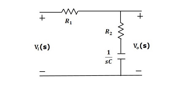
Here, the capacitor is in series with the resistor $R_2$ and the output is measured across this combination.

The transfer function of this lag compensator is -

$$\frac{V_o(s)}{V_i(s)}=\frac{1}{\alpha} \left( \frac{s+\frac{1}{\tau}}{s+\frac{1}{\alpha\tau}} \right )$$

Where,

$$\tau=R_2C$$

$$\alpha=\frac{R_1+R_2}{R_2}$$

From the above equation, $\alpha$ is always greater than one.

From the transfer function, we can conclude that the lag compensator has one pole at $s = − \frac{1}{\alpha \tau}$ and one zero at $s = −\frac{1}{\tau}$ . This means, the pole will be nearer to origin in the pole-zero configuration of the lag compensator.

Substitute, $s = j\omega$ in the transfer function.

$$\frac{V_o(j\omega)}{V_i(j\omega)}=\frac{1}{\alpha}\left( \frac{j\omega+\frac{1}{\tau}}{j\omega+\frac{1}{\alpha\tau}}\right )$$

Phase angle $\phi = \tan^{−1} \omega\tau − tan^{−1} \alpha\omega\tau$

We know that, the phase of the output sinusoidal signal is equal to the sum of the phase angles of input sinusoidal signal and the transfer function.

So, in order to produce the phase lag at the output of this compensator, the phase angle of the transfer function should be negative. This will happen when $\alpha > 1$.

Lead Compensator

The lead compensator is an electrical network which produces a sinusoidal output having phase lead when a sinusoidal input is applied. The lead compensator circuit in the ‘s’ domain is shown in the following figure.

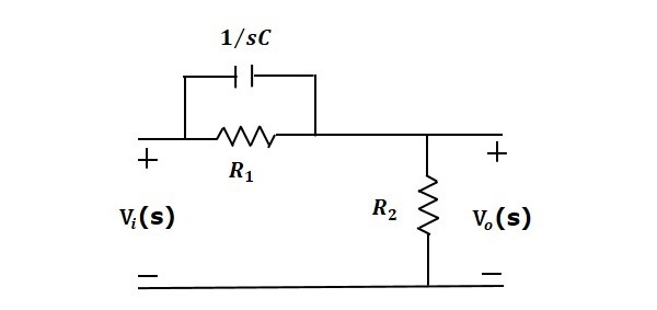
Here, the capacitor is parallel to the resistor $R_1$ and the output is measured across resistor $R_2.

The transfer function of this lead compensator is -

$$\frac{V_o(s)}{V_i(s)}=\beta \left( \frac{s\tau+1}{\beta s\tau+1} \right )$$

Where,

$$\tau=R_1C$$

$$\beta=\frac{R_2}{R_1+R_2}$$

From the transfer function, we can conclude that the lead compensator has pole at $s = −\frac{1}{\beta}$ and zero at $s = − \frac{1}{\beta\tau}$.

Substitute, $s = j\omega$ in the transfer function.

$$\frac{V_o(j\omega)}{V_i(j\omega)}=\beta \left( \frac{j\omega\tau+1}{\beta j \omega\tau+1} \right )$$

Phase angle $\phi = tan^{−1}\omega\tau − tan^{−1}\beta\omega\tau$

We know that, the phase of the output sinusoidal signal is equal to the sum of the phase angles of input sinusoidal signal and the transfer function.

So, in order to produce the phase lead at the output of this compensator, the phase angle of the transfer function should be positive. This will happen when $0 < \beta < 1$. Therefore, zero will be nearer to origin in pole-zero configuration of the lead compensator.

Lag-Lead Compensator

Lag-Lead compensator is an electrical network which produces phase lag at one frequency region and phase lead at other frequency region. It is a combination of both the lag and the lead compensators. The lag-lead compensator circuit in the ‘s’ domain is shown in the following figure.

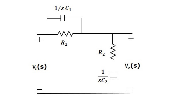
This circuit looks like both the compensators are cascaded. So, the transfer function of this circuit will be the product of transfer functions of the lead and the lag compensators.

$$\frac{V_o(s)}{V_i(s)}=\beta \left( \frac{s\tau_1+1}{\beta s \tau_1+1} \right )\frac{1}{\alpha} \left ( \frac{s+\frac{1}{\tau_2}}{s+\frac{1}{\alpha\tau_2}} \right )$$

We know $\alpha\beta=1$.

$$\Rightarrow \frac{V_o(s)}{V_i(s)}=\left ( \frac{s+\frac{1}{\tau_1}}{s+\frac{1}{\beta\tau_1}} \right )\left ( \frac{s+\frac{1}{\tau_2}}{s+\frac{1}{\alpha\tau_2}} \right )$$

Where,

$$\tau_1=R_1C_1$$

$$\tau_2=R_2C_2$$