- Control Systems - Home
- Control Systems - Introduction
- Control Systems - Feedback
- Mathematical Models
- Modelling of Mechanical Systems
- Electrical Analogies of Mechanical Systems
- Control Systems - Block Diagrams
- Block Diagram Algebra
- Block Diagram Reduction
- Signal Flow Graphs
- Mason's Gain Formula
- Time Response Analysis
- Response of the First Order System
- Response of Second Order System
- Time Domain Specifications
- Steady State Errors
- Control Systems - Stability
- Control Systems - Stability Analysis
- Control Systems - Root Locus
- Construction of Root Locus
- Frequency Response Analysis
- Control Systems - Bode Plots
- Construction of Bode Plots
- Control Systems - Polar Plots
- Control Systems - Nyquist Plots
- Control Systems - Compensators
- Control Systems - Controllers
- Control Systems - State Space Model
- State Space Analysis
Control Systems - Block Diagram Algebra
Block diagram algebra is nothing but the algebra involved with the basic elements of the block diagram. This algebra deals with the pictorial representation of algebraic equations.
Basic Connections for Blocks
There are three basic types of connections between two blocks.
Series Connection
Series connection is also called cascade connection. In the following figure, two blocks having transfer functions $G_1(s)$ and $G_2(s)$ are connected in series.
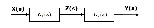
For this combination, we will get the output $Y(s)$ as
$$Y(s)=G_2(s)Z(s)$$
Where, $Z(s)=G_1(s)X(s)$
$$\Rightarrow Y(s)=G_2(s)[G_1(s)X(s)]=G_1(s)G_2(s)X(s)$$
$$\Rightarrow Y(s)=\lbrace G_1(s)G_2(s)\rbrace X(s)$$
Compare this equation with the standard form of the output equation, $Y(s)=G(s)X(s)$. Where, $G(s) = G_1(s)G_2(s)$.
That means we can represent the series connection of two blocks with a single block. The transfer function of this single block is the product of the transfer functions of those two blocks. The equivalent block diagram is shown below.

Similarly, you can represent series connection of n blocks with a single block. The transfer function of this single block is the product of the transfer functions of all those n blocks.
Parallel Connection
The blocks which are connected in parallel will have the same input. In the following figure, two blocks having transfer functions $G_1(s)$ and $G_2(s)$ are connected in parallel. The outputs of these two blocks are connected to the summing point.
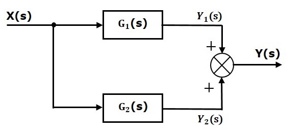
For this combination, we will get the output $Y(s)$ as
$$Y(s)=Y_1(s)+Y_2(s)$$
Where, $Y_1(s)=G_1(s)X(s)$ and $Y_2(s)=G_2(s)X(s)$
$$\Rightarrow Y(s)=G_1(s)X(s)+G_2(s)X(s)=\lbrace G_1(s)+G_2(s)\rbrace X(s)$$
Compare this equation with the standard form of the output equation, $Y(s)=G(s)X(s)$.
Where, $G(s)=G_1(s)+G_2(s)$.
That means we can represent the parallel connection of two blocks with a single block. The transfer function of this single block is the sum of the transfer functions of those two blocks. The equivalent block diagram is shown below.

Similarly, you can represent parallel connection of n blocks with a single block. The transfer function of this single block is the algebraic sum of the transfer functions of all those n blocks.
Feedback Connection
As we discussed in previous chapters, there are two types of feedback positive feedback and negative feedback. The following figure shows negative feedback control system. Here, two blocks having transfer functions $G(s)$ and $H(s)$ form a closed loop.
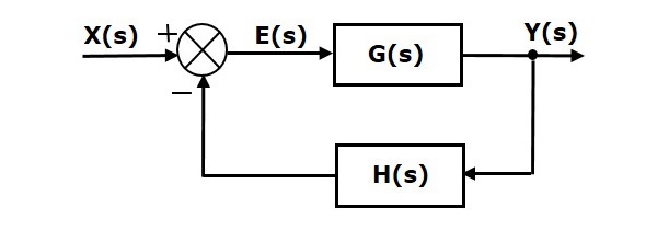
The output of the summing point is -
$$E(s)=X(s)-H(s)Y(s)$$
The output $Y(s)$ is -
$$Y(s)=E(s)G(s)$$
Substitute $E(s)$ value in the above equation.
$$Y(s)=\left \{ X(s)-H(s)Y(s)\rbrace G(s) \right\}$$
$$Y(s)\left \{ 1+G(s)H(s)\rbrace = X(s)G(s) \right\}$$
$$\Rightarrow \frac{Y(s)}{X(s)}=\frac{G(s)}{1+G(s)H(s)}$$
Therefore, the negative feedback closed loop transfer function is $\frac{G(s)}{1+G(s)H(s)}$
This means we can represent the negative feedback connection of two blocks with a single block. The transfer function of this single block is the closed loop transfer function of the negative feedback. The equivalent block diagram is shown below.
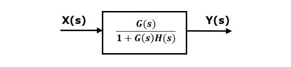
Similarly, you can represent the positive feedback connection of two blocks with a single block. The transfer function of this single block is the closed loop transfer function of the positive feedback, i.e., $\frac{G(s)}{1-G(s)H(s)}$
Block Diagram Algebra for Summing Points
There are two possibilities of shifting summing points with respect to blocks −
- Shifting summing point after the block
- Shifting summing point before the block
Let us now see what kind of arrangements need to be done in the above two cases one by one.
Shifting Summing Point After the Block
Consider the block diagram shown in the following figure. Here, the summing point is present before the block.
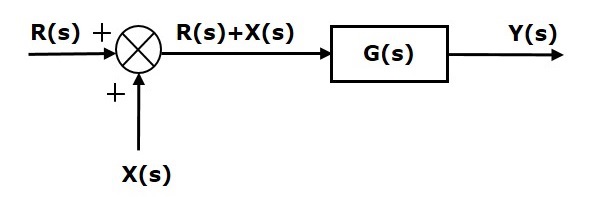
Summing point has two inputs $R(s)$ and $X(s)$. The output of it is $\left \{R(s)+X(s)\right\}$.
So, the input to the block $G(s)$ is $\left \{R(s)+X(s)\right \}$ and the output of it is
$$Y(s)=G(s)\left \{R(s)+X(s)\right \}$$
$\Rightarrow Y(s)=G(s)R(s)+G(s)X(s)$ (Equation 1)
Now, shift the summing point after the block. This block diagram is shown in the following figure.
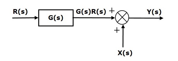
Output of the block $G(s)$ is $G(s)R(s)$.
The output of the summing point is
$Y(s)=G(s)R(s)+X(s)$ (Equation 2)
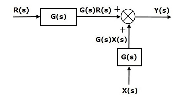
Compare Equation 1 and Equation 2.
The first term $G(s) R(s)$ is same in both the equations. But, there is difference in the second term. In order to get the second term also same, we require one more block $G(s)$. It is having the input $X(s)$ and the output of this block is given as input to summing point instead of $X(s)$. This block diagram is shown in the following figure.
Shifting Summing Point Before the Block
Consider the block diagram shown in the following figure. Here, the summing point is present after the block.
Output of this block diagram is -
$Y(s)=G(s)R(s)+X(s)$ (Equation 3)
Now, shift the summing point before the block. This block diagram is shown in the following figure.
Output of this block diagram is -
$Y(S)=G(s)R(s)+G(s)X(s)$ (Equation 4)
Compare Equation 3 and Equation 4,
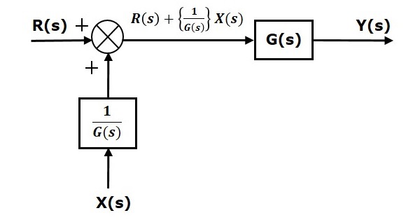
The first term $G(s) R(s)$ is same in both equations. But, there is difference in the second term. In order to get the second term also same, we require one more block $\frac{1}{G(s)}$. It is having the input $X(s)$ and the output of this block is given as input to summing point instead of $X(s)$. This block diagram is shown in the following figure.
Block Diagram Algebra for Take-off Points
There are two possibilities of shifting the take-off points with respect to blocks −
- Shifting take-off point after the block
- Shifting take-off point before the block
Let us now see what kind of arrangements are to be done in the above two cases, one by one.
Shifting Take-off Point After the Block
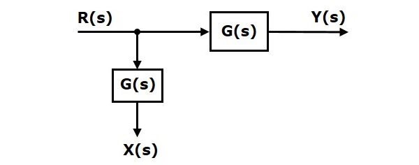
Consider the block diagram shown in the following figure. In this case, the take-off point is present before the block.
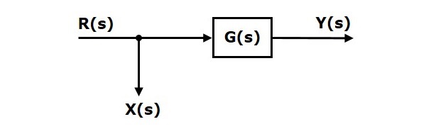
Here, $X(s)=R(s)$ and $Y(s)=G(s)R(s)$
When you shift the take-off point after the block, the output $Y(s)$ will be same. But, there is difference in $X(s)$ value. So, in order to get the same $X(s)$ value, we require one more block $\frac{1}{G(s)}$. It is having the input $Y(s)$ and the output is $X(s)$. This block diagram is shown in the following figure.
Shifting Take-off Point Before the Block
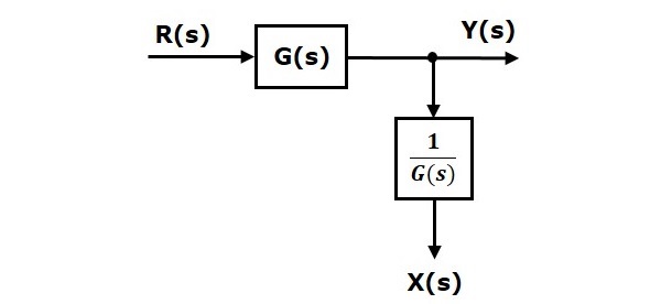
Consider the block diagram shown in the following figure. Here, the take-off point is present after the block.
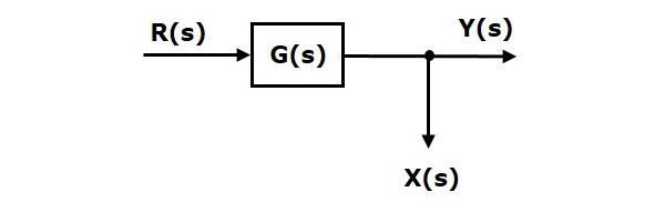
Here, $X(s)=Y(s)=G(s)R(s)$
When you shift the take-off point before the block, the output $Y(s)$ will be same. But, there is difference in $X(s)$ value. So, in order to get same $X(s)$ value, we require one more block $G(s)$. It is having the input $R(s)$ and the output is $X(s)$. This block diagram is shown in the following figure.