Plotly - Subplots and Inset Plots

---

Here, we will understand the concept of subplots and inset plots in Plotly.

Making Subplots

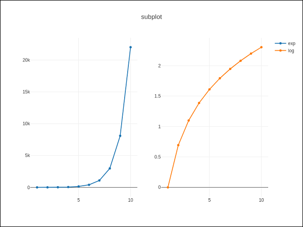
Sometimes it is helpful to compare different views of data side by side. This supports the concept of subplots. It offers make_subplots() function in plotly.tools module. The function returns a Figure object.

The following statement creates two subplots in one row.

fig = tools.make_subplots(rows = 1, cols = 2)

We can now add two different traces (the exp and log traces in example above) to the figure.

fig.append_trace(trace1, 1, 1)
fig.append_trace(trace2, 1, 2)

The Layout of figure is further configured by specifying title, width, height, etc. using update() method.

fig['layout'].update(height = 600, width = 800s, title = 'subplots')

Here's the complete script −

from plotly import tools
import plotly.plotly as py
import plotly.graph_objs as go
from plotly.offline import iplot, init_notebook_mode
init_notebook_mode(connected = True)
import numpy as np
x = np.arange(1,11)
y1 = np.exp(x)
y2 = np.log(x)
trace1 = go.Scatter(
   x = x,
   y = y1,
   name = 'exp'
)
trace2 = go.Scatter(
   x = x,
   y = y2,
   name = 'log'
)
fig = tools.make_subplots(rows = 1, cols = 2)
fig.append_trace(trace1, 1, 1)
fig.append_trace(trace2, 1, 2)
fig['layout'].update(height = 600, width = 800, title = 'subplot')
iplot(fig)

This is the format of your plot grid: [ (1,1) x1,y1 ] [ (1,2) x2,y2 ]

Inset Plots

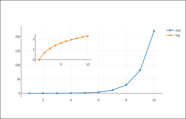
To display a subplot as inset, we need to configure its trace object. First the xaxis and yaxis properties of inset trace to ‘x2’ and ‘y2’ respectively. Following statement puts ‘log’ trace in inset.

trace2 = go.Scatter(
   x = x,
   y = y2,
   xaxis = 'x2',
   yaxis = 'y2',
   name = 'log'
)

Secondly, configure Layout object where the location of x and y axes of inset is defined by domain property that specifies is position with respective to major axis.

xaxis2=dict(
   domain = [0.1, 0.5],
   anchor = 'y2'
),
yaxis2 = dict(
   domain = [0.5, 0.9],
   anchor = 'x2'
)

Complete script to display log trace in inset and exp trace on main axis is given below −

trace1 = go.Scatter(
   x = x,
   y = y1,
   name = 'exp'
)
trace2 = go.Scatter(
   x = x,
   y = y2,
   xaxis = 'x2',
   yaxis = 'y2',
   name = 'log'
)
data = [trace1, trace2]
layout = go.Layout(
   yaxis = dict(showline = True),
   xaxis2 = dict(
      domain = [0.1, 0.5],
      anchor = 'y2'
   ),
   yaxis2 = dict(
      showline = True,
      domain = [0.5, 0.9],
      anchor = 'x2'
   )
)
fig = go.Figure(data=data, layout=layout)
iplot(fig)

The output is mentioned below −