
Article Categories
- All Categories
-
 Data Structure
-
 Networking
-
 RDBMS
RDBMS
-
 Operating System
-
 Java
Java
-
 MS Excel
-
 iOS
iOS
-
 HTML
HTML
-
 CSS
CSS
-
 Android
-
 Python
-
 C Programming
-
 C++
C++
-
 C#
C#
-
 MongoDB
-
 MySQL
MySQL
-
 Javascript
-
 PHP
PHP
-
 Economics & Finance
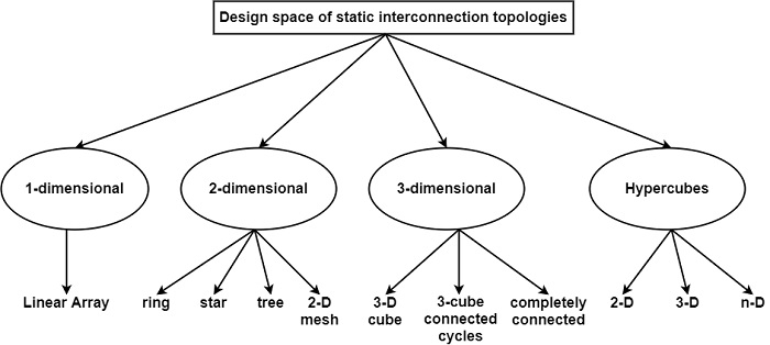
What is design space of static interconnection topology?
In a static network, the connection between input and output nodes is fixed and cannot be modified. Static interconnection network cannot be reconfigured. Examples of this network are linear array, ring, chordal ring, tree, star, fat tree, mesh, tours, systolic arrays, and hypercube. The design space for static interconnection topologies is shown in the figure.
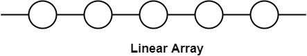
Linear Array
This is a most elementary interconnection design. In this processors are linked in a linear one-dimensional array. The first and last processors are linked with one adjacent processor and the middle processing components are linked with two adjacent processors. It is a one-dimensional interconnection network.
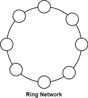
Ring
This is a simple linear array where the end nodes are linked. It is similar to a mesh with wrap-around connections. The data transfer in a ring is generally in one direction.
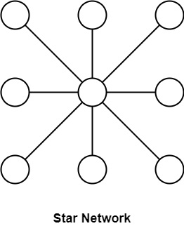
Star
The star connection is another simple and low-cost (C=N-1) topology as shown in the figure which has the same poor bisection width (B=1) and arc connectivity (A=1) parameters as the linear array but the diameter is radically improved (D=2).
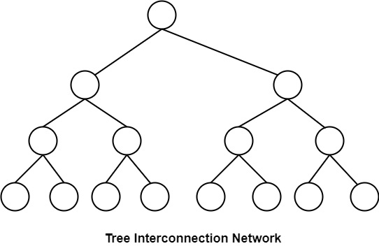
Tree interconnection network
In the tree interconnection network, processors are organized in a complete binary tree scheme.
Fat tree
It is a changed version of the tree network. In this network, the bandwidth of the edge improves towards the root. It is a more sensible simulation of the normal tree where branches get deep towards the root.
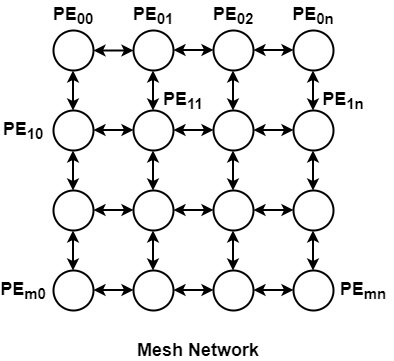
2-D Mesh
It is a two-dimensional network. In this, all processing components are organized in a two-dimensional grid. The processor in rows i and column j are indicated by PEi.
The processors on the corner can connect to two nearest neighbors i.e. PE00 can connect with PE01 and PE10. The processor on the boundary can connect to 3 adjacent processing elements i.e. PE01 can interact with PE00, PE02, and PE11 and internally placed processors can connect with 4 adjacent processors i.e. PE11 can connect with PE01, PE10, PE12, and PE21.
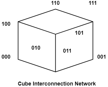
3-D Cube
It is a 3-dimensional interconnection network. In this, the PE’s are organized in a cube structure.
HyperCube
A Hypercube interconnection network is an extension of a cube network. Hypercube interconnection network for n ≥ 3, can be represented recursively as follows −
For n = 3, it cube network in which nodes are assigned number 0, 1… 7 in binary. In other words, one of the nodes is assigned a label 000, another one as 001…. and the final node is 111.
Thus any node can connect with any other node if their labels differ in exactly one place, e.g., the node with label 101 can connect directly with 001, 000, and 111.
Completely Connected Network
This topology is ideal from the point of view of network diameter (D=1) since any two nodes are directly connected. The cost (C=N (N-1)/2) and node degree (d=N-1) parameters are prohibitive in building massively parallel computers based on this topology.

2K+ Views
