- Home
- Adjusted R-Squared
- Analysis of Variance
- Arithmetic Mean
- Arithmetic Median
- Arithmetic Mode
- Arithmetic Range
- Bar Graph
- Best Point Estimation
- Beta Distribution
- Binomial Distribution
- Black-Scholes model
- Boxplots
- Central limit theorem
- Chebyshev's Theorem
- Chi-squared Distribution
- Chi Squared table
- Circular Permutation
- Cluster sampling
- Cohen's kappa coefficient
- Combination
- Combination with replacement
- Comparing plots
- Continuous Uniform Distribution
- Continuous Series Arithmetic Mean
- Continuous Series Arithmetic Median
- Continuous Series Arithmetic Mode
- Cumulative Frequency
- Co-efficient of Variation
- Correlation Co-efficient
- Cumulative plots
- Cumulative Poisson Distribution
- Data collection
- Data collection - Questionaire Designing
- Data collection - Observation
- Data collection - Case Study Method
- Data Patterns
- Deciles Statistics
- Discrete Series Arithmetic Mean
- Discrete Series Arithmetic Median
- Discrete Series Arithmetic Mode
- Dot Plot
- Exponential distribution
- F distribution
- F Test Table
- Factorial
- Frequency Distribution
- Gamma Distribution
- Geometric Mean
- Geometric Probability Distribution
- Goodness of Fit
- Grand Mean
- Gumbel Distribution
- Harmonic Mean
- Harmonic Number
- Harmonic Resonance Frequency
- Histograms
- Hypergeometric Distribution
- Hypothesis testing
- Individual Series Arithmetic Mean
- Individual Series Arithmetic Median
- Individual Series Arithmetic Mode
- Interval Estimation
- Inverse Gamma Distribution
- Kolmogorov Smirnov Test
- Kurtosis
- Laplace Distribution
- Linear regression
- Log Gamma Distribution
- Logistic Regression
- Mcnemar Test
- Mean Deviation
- Means Difference
- Multinomial Distribution
- Negative Binomial Distribution
- Normal Distribution
- Odd and Even Permutation
- One Proportion Z Test
- Outlier Function
- Permutation
- Permutation with Replacement
- Pie Chart
- Poisson Distribution
- Pooled Variance (r)
- Power Calculator
- Probability
- Probability Additive Theorem
- Probability Multiplecative Theorem
- Probability Bayes Theorem
- Probability Density Function
- Process Capability (Cp) & Process Performance (Pp)
- Process Sigma
- Quadratic Regression Equation
- Qualitative Data Vs Quantitative Data
- Quartile Deviation
- Range Rule of Thumb
- Rayleigh Distribution
- Regression Intercept Confidence Interval
- Relative Standard Deviation
- Reliability Coefficient
- Required Sample Size
- Residual analysis
- Residual sum of squares
- Root Mean Square
- Sample planning
- Sampling methods
- Scatterplots
- Shannon Wiener Diversity Index
- Signal to Noise Ratio
- Simple random sampling
- Skewness
- Standard Deviation
- Standard Error ( SE )
- Standard normal table
- Statistical Significance
- Statistics Formulas
- Statistics Notation
- Stem and Leaf Plot
- Stratified sampling
- Student T Test
- Sum of Square
- T-Distribution Table
- Ti 83 Exponential Regression
- Transformations
- Trimmed Mean
- Type I & II Error
- Variance
- Venn Diagram
- Weak Law of Large Numbers
- Z table
- Statistics Useful Resources
- Statistics - Discussion
Statistics - Residual analysis
Residual analysis is used to assess the appropriateness of a linear regression model by defining residuals and examining the residual plot graphs.
Residual
Residual($ e $) refers to the difference between observed value($ y $) vs predicted value ($ \hat y $). Every data point have one residual.
${ residual = observedValue - predictedValue \\[7pt] e = y - \hat y }$
Residual Plot
A residual plot is a graph in which residuals are on tthe vertical axis and the independent variable is on the horizontal axis. If the dots are randomly dispersed around the horizontal axis then a linear regression model is appropriate for the data; otherwise, choose a non-linear model.
Types of Residual Plot
Following example shows few patterns in residual plots.
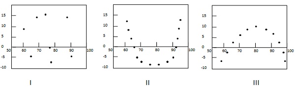
In first case, dots are randomly dispersed. So linear regression model is preferred. In Second and third case, dots are non-randomly dispersed and suggests that a non-linear regression method is preferred.
Example
Problem Statement:
Check where a linear regression model is appropriate for the following data.
| $ x $ | 60 | 70 | 80 | 85 | 95 |
|---|---|---|---|---|---|
| $ y $ (Actual Value) | 70 | 65 | 70 | 95 | 85 |
| $ \hat y $ (Predicted Value) | 65.411 | 71.849 | 78.288 | 81.507 | 87.945 |
Solution:
Step 1: Compute residuals for each data point.
| $ x $ | 60 | 70 | 80 | 85 | 95 |
|---|---|---|---|---|---|
| $ y $ (Actual Value) | 70 | 65 | 70 | 95 | 85 |
| $ \hat y $ (Predicted Value) | 65.411 | 71.849 | 78.288 | 81.507 | 87.945 |
| $ e $ (Residual) | 4.589 | -6.849 | -8.288 | 13.493 | -2.945 |
Step 2: - Draw the residual plot graph.
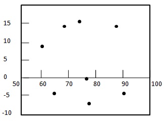
Step 3: - Check the randomness of the residuals.
Here residual plot exibits a random pattern - First residual is positive, following two are negative, the fourth one is positive, and the last residual is negative. As pattern is quite random which indicates that a linear regression model is appropriate for the above data.
