
Article Categories
- All Categories
-
 Data Structure
-
 Networking
-
 RDBMS
RDBMS
-
 Operating System
-
 Java
Java
-
 MS Excel
-
 iOS
iOS
-
 HTML
HTML
-
 CSS
CSS
-
 Android
-
 Python
-
 C Programming
-
 C++
C++
-
 C#
C#
-
 MongoDB
-
 MySQL
MySQL
-
 Javascript
-
 PHP
PHP
-
 Economics & Finance
How to group ages in ranges with VLOOKUP in Excel?
VLOOKUP is a function in Microsoft Excel mostly used to search for a specific value in the first column of a table and then retrieve a corresponding value from a different column in the same row. The name "VLOOKUP" stands for "Vertical Lookup". This simply means that the function looks up a value vertically within a table. This article will use user defined VLOOK formula, to determine the age group for provided age data.
The article briefs all the steps accurately and precisely. Grouping data in Excel allows for improving the organization of data and makes data easier to read and analyze. Another major factor is that it makes the data manipulation easy. This means that modification and alteration of data become easy. Grouping also simplifies the process of Data Analysis. In short, while dealing with large data sets, using a group is a very worthy option.
To group ages in ranges with VLOOKUP in Excel by using the user-defined formula
Step 1
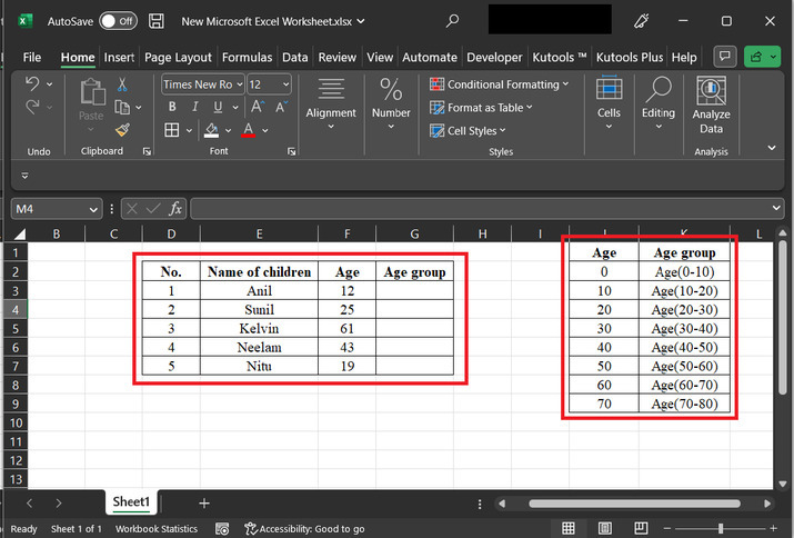
Consider the given worksheet below. This worksheet contains two tables. The first table contains 4 column fields. The second column contains "name of children". The third column contains the age of the children. 4 th column contains the space for the data. The second table contains the age data, and the second column contains the age group of the user.
Step 2
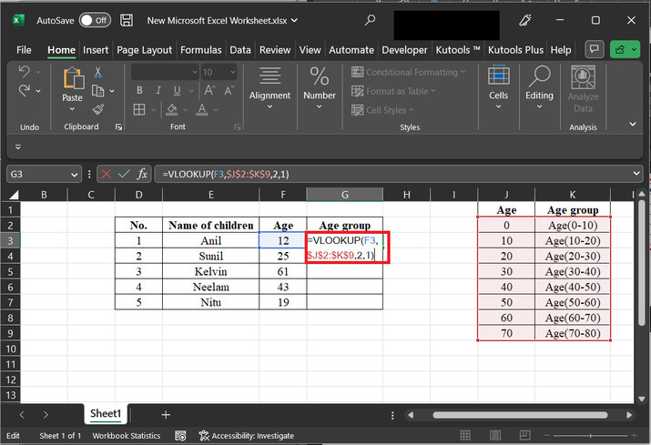
Now, go to the "G3" cell, and type the below-given formula
"=VLOOKUP(F3,$J$2:$K$9,2,1)".
Explanation for the above formula
The VLOOKUP formula is used in Excel to search for a specific value in the leftmost column of a table, and then return a corresponding value from a specified column in the same row of that table.
"F3" is the value that the user wants to search for in the leftmost column of the table.
"$J$2:$K$9" is the range of cells that contains the table from where the user wants to retrieve the corresponding value. In this case, the table is located in cells J2:K9.
"2" specifies the column number (in the table) from where the user wants to retrieve the corresponding value. In this case, the user wants to retrieve the value from the second column of the table (column K).
"1" indicates that the user wants to determine an approximate match. This means that if an exact match for the value in F3 is not found in the leftmost column of the table, the formula will return the closest match that is less than the lookup value.
Consider the below-given code snapshot for proper reference ?
Please note that the user needs to set the column name and rage data according to the data chosen for processing. The provided formula is a good match for taken data, but, for new data, the user needs to change the available values accordingly.
Step 3
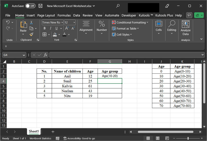
Consider the below-provided output snapshot for proper reference ?
Step 4
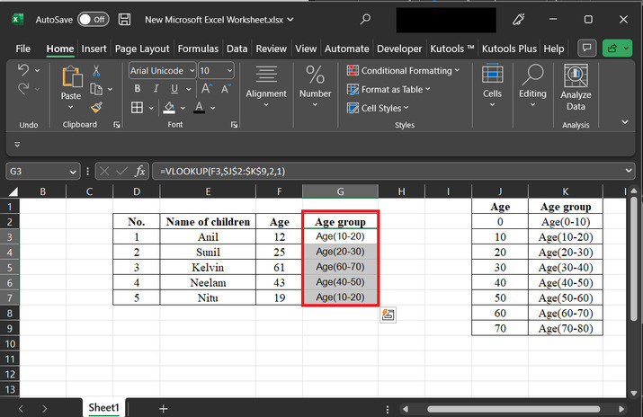
Click on the bottom of the G3 cell. this area contains a "plus" sign. Simply, drag the "plus" cell to the bottom of the cell, to copy the formula for other rows. The final generated code snapshot is given below ?
Conclusion
After successful completion of all the steps, the learner will be able to replace the age with the appropriate age group, as guided above. The provided article contains a brief and stepwise explanation of all the steps. All the provided steps are thorough and well-explained and can be easily leaner by a beginner as well.

5K+ Views
