
Article Categories
- All Categories
-
 Data Structure
-
 Networking
-
 RDBMS
RDBMS
-
 Operating System
-
 Java
Java
-
 MS Excel
-
 iOS
iOS
-
 HTML
HTML
-
 CSS
CSS
-
 Android
-
 Python
-
 C Programming
-
 C++
C++
-
 C#
C#
-
 MongoDB
-
 MySQL
MySQL
-
 Javascript
-
 PHP
PHP
-
 Economics & Finance
How to Apply Conditional Formatting based on VLOOKUP in Excel?
Have you ever tried comparing the data on two different work sheets? Yes, it is possible to compare data from two different sheets in Excel. Let us assume we have two lists that contain the current prices of stocks and the price of a stock last month for a list of stocks, and you want to compare them to know where the price is high. In this tutorial, we will help you understand how you can apply conditional formatting based on VLOOKUP in Excel.
Applying Conditional Formatting based on VLOOKUP
Here we will apply the conditional formatting to cells based on the cell value. Let's take a look at a simple procedure for applying conditional formatting in Excel using VLOOKUP. We will be using the VLOOKUP function as a formatting formula.
Step 1
Let us consider that we have two work sheets that contain data similar to the data shown below.
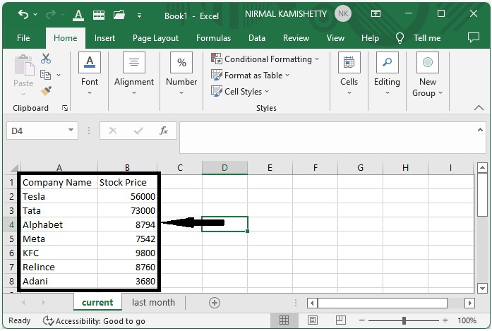
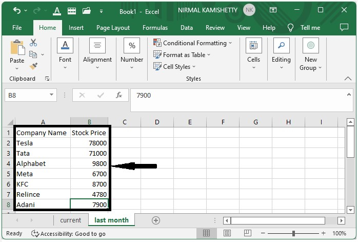
Step 2
Now, in the current sheet, select the data, then click on the conditional formatting and select a new rule under "Home" in the Excel ribbon, which will open a new pop-up window similar to the one shown below.
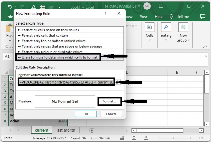
Step 3
Now in the new pop-up, select Use the Formula and enter the formula as
=VLOOKUP($A2,'last month'!$A$1:$B$8,2,FALSE) < current!$B2 in the formula box and click on format, then select the colour you want to use and click OK to close both pop-ups, and our final result will look like the screenshot below.
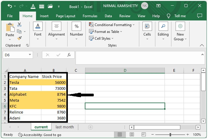
As we can see, we successfully highlighted the companies whose stock price has decreased compared to the last month.
Conclusion
In this tutorial, we used a simple example to demonstrate how you can apply conditional formatting based on VLOOKUP in Excel to highlight a particular set of data.

5K+ Views
