
Article Categories
- All Categories
-
 Data Structure
-
 Networking
-
 RDBMS
RDBMS
-
 Operating System
-
 Java
Java
-
 MS Excel
-
 iOS
iOS
-
 HTML
HTML
-
 CSS
CSS
-
 Android
-
 Python
-
 C Programming
-
 C++
C++
-
 C#
C#
-
 MongoDB
-
 MySQL
MySQL
-
 Javascript
-
 PHP
PHP
-
 Economics & Finance
How to rank values by group in excel?
Excel's ranking values by group function aims to rank data points inside particular groupings or categories. With the use of this method, you can ascertain the relative locations and rankings of the data points inside each group, allowing you to compare and analyze the data depending on how each group ranks the different data points. Comparing values within each group and highlighting the top and lowest values within each category or subset are made possible by grouping values. This makes it easier to identify the best performers, outliers, or patterns unique to each group, offering insightful information for making decisions or conducting additional research.
Excel's ability to rank values by group enables targeted analysis, within-group comparisons, and contextual ranking, aiding decision-making based on the rankings within particular groups or categories.
Example 1: To Find Rank Data by Alphabetical Order in Excel
Step 1
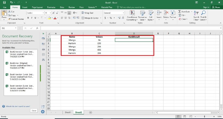
In the first step, users have created the three fields i.,e Name, Values, and Rank Result. Following is the screenshot of this step.
Step 2
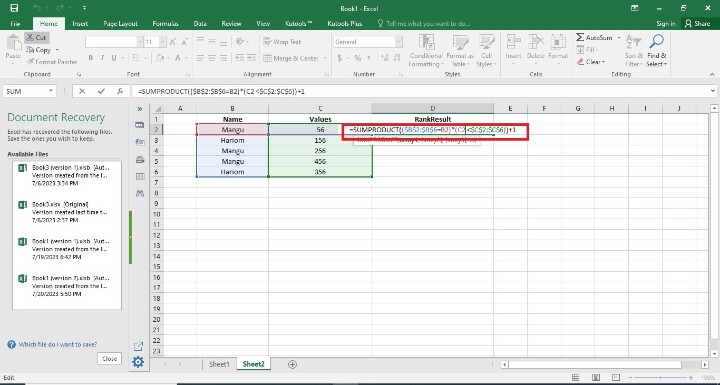
In the previous step, the user has created the three columns in this step user has entered the formula in the D2 Cell i.e =SUMPRODUCT(($B$2:$B$6=B2)*(C2 <$C$2:$C$6))+1. Following is the screenshot of this step.
Explanation
=SUMPRODUCT(($B$2:$B$6=B2)*(C2 <$C$2:$C$6))+1
The equation, ($B$2:$B$6=B2)*(C2 $C$2:$C$6), is =SUMPRODUCT(($B$2:$B$6))+1.
In Excel, it is used to determine the rank of a particular value inside a group based on a particular set of criteria. Let's examine the formula in detail ?
The range of columns in column B where you are doing the comparison to the value in cell B2 is $B$2:$B$6.
The formula =B2 gives an array of TRUE or FALSE values after comparing each cell in the range $B$2:$B$6 to the value in cell B2.
(C2 $C$2:$C$6) generates an array of TRUE or FALSE values by comparing the value in cell C2 to each cell in the $C$2:$C$6 range.
($B$2:$B$6=B2) means the two arrays are multiplied element-by-element by *(C2 $C$2:$C$6), producing an array with TRUE values when both requirements are met and FALSE values in all other cases.
The SUMPRODUCT function adds up the array's values, counting how many of them are TRUE.
+1 increases the total by one, signifying the rank.
Step 3
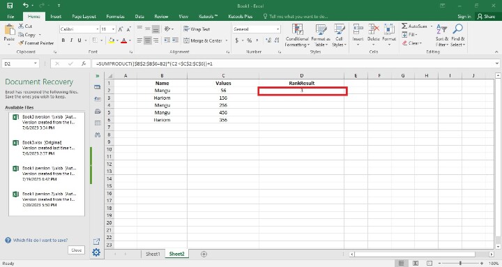
In this step, users have to press the Enter Button. Following is the screenshot of this step.
Step 4
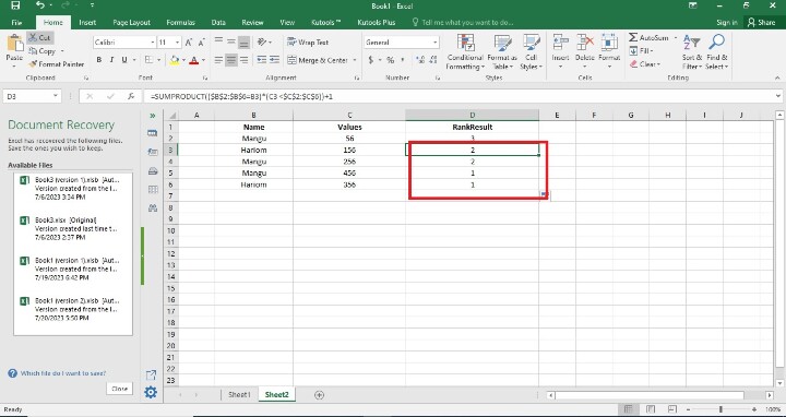
In this step, users have to find the remaining Rank Result result cells. It may be done in two ways. The first way is that users have written the formula in each cell by writing its initial value. The second way is a simple way here users have only drag the fill handle to the final cell. Following is the screenshot of this step.
Conclusion
In conclusion, Excel's ranking values by group feature offers an effective tool for examining and contrasting data across different categories or subsets. Users can set the relative positions and rankings of data items by allocating ranks inside each group, providing targeted analysis, within-group comparisons, and contextual ranking.
Gaining knowledge about the relative positions and rankings of data points within particular categories or subsets is the goal of ranking values by group. Given that it takes into account the distinctive traits and dynamics of each group within the dataset, this method enables a more targeted analysis.

2K+ Views
