How to Rename Group or Row Labels in Excel PivotTable?

Excel's pivot tables are strong tools that make it simple to analyse and summarise huge datasets. They give you the ability to easily manipulate and meaningfully present your data. Managing the labels that organise and categorise your data is a crucial part of using PivotTables.

You will learn how to rename group or row labels in an Excel pivot table in this article. Sometimes, the Excel default labels may not be sufficiently descriptive or may need to be customised to meet your unique reporting requirements. You may make a PivotTable that better explains your data analysis and is more user-friendly by knowing how to rename these labels.

Rename Group or Row Labels in Excel PivotTable

Here we will complete the task using the methods mentioned in this tutorial. So let us see a simple process to know how you can rename group or row labels in Excel PivotTable.

Step 1

Consider an Excel sheet where you have a pivot table similar to the below image.

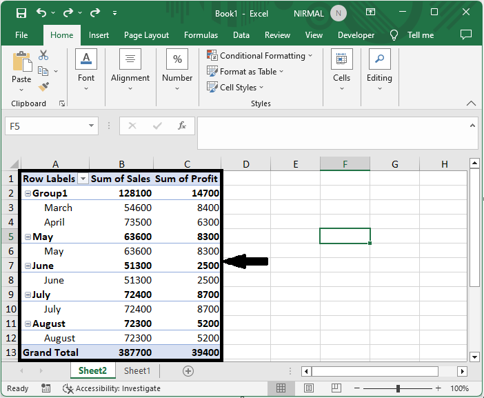
First, to rename the group name, click on the cell containing the group name, edit the name using the formula box, and click enter.

Cell > Rename > Enter.

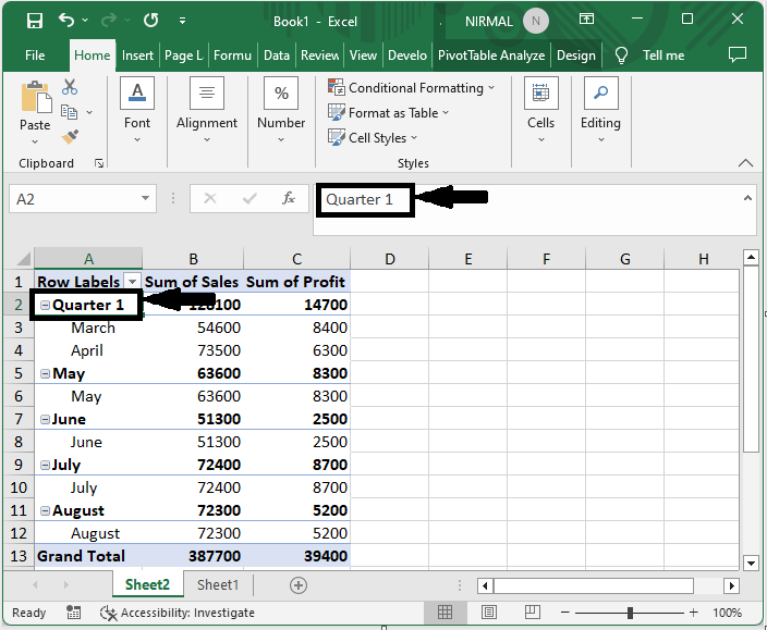
This is how you can rename groups in Excel.

Step 2

Now to rename the row label, click on any cell of the row, click on analyse, edit the name under the active field, and click enter.

Cell > Analyse > Active Field > Enter.

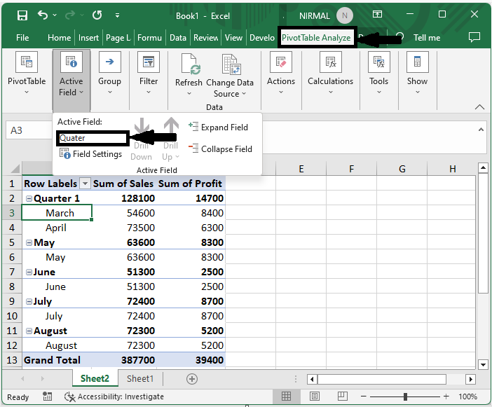
Then you will see that the row label will be renamed. This is how you can rename row labels and group labels in Excel.

Conclusion

In this tutorial, we have used a simple example to demonstrate how you can rename group or row labels in an Excel pivot table to highlight a particular set of data.

Pradeep Kumar

e

Updated on: 13-Sep-2023

2K+ Views

Kickstart Your Career

Get certified by completing the course

Get Started