How to hide or display cells with zero values in selected ranges in Excel?

In Excel, users sometimes want to display cells with zero values as blanks rather than hiding them from view. One may or may not need zero (0) numbers to be visible on the worksheets depending on the situation. There are several methods to make zeroes visible or hidden, depending on the format's standards or preferences.

How do we show a zero value in Excel when we need to? This article concentrates on ways to make Excel worksheet cells with zero values invisible or visible.

In this article, learners will understand the simplest practice to hide or display cells with zero values in a selected range. This article contains two examples that contain sufficient explanations for learners, along with detailed explanations, and proper output snapshots.

Example 1: To hide available zero value from the selected range in Excel

Step 1

To understand the process of hiding the 0, available in the provided Excel sheet. Firstly, select the cell range as specified below. The provided data contains 9 numeric values with 0.

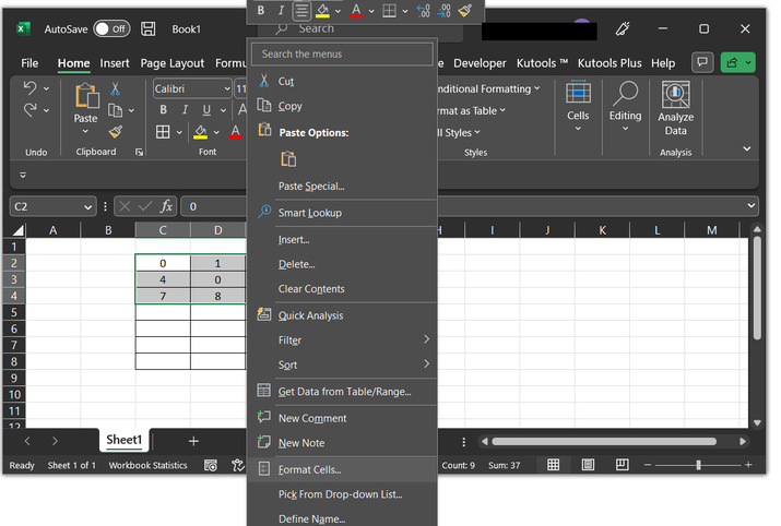
Step 2

Now right-click on the selected range. This will display a drop-down menu. Consider below provided snapshot for proper reference −

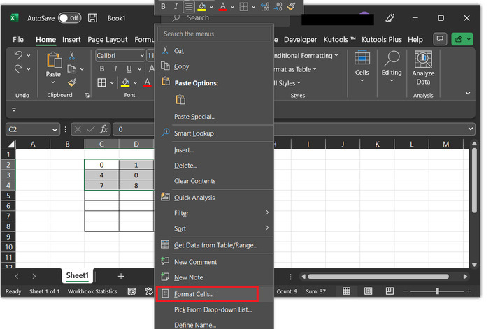
Step 3

Now click on “Format Cells” options.

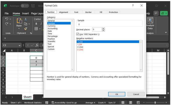
Step 4

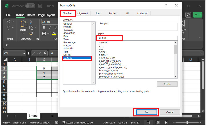
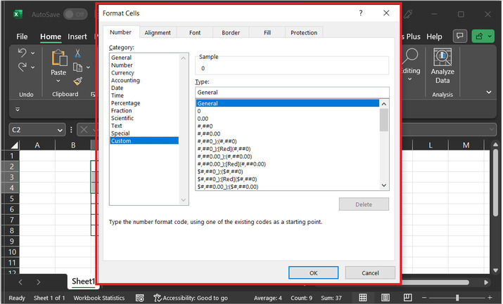
This will display the “Format cells” dialog box, as provided below.

Step 5

Under the Number tab go to the “Custom” section. Consider all the stepwise snapshots to understand the data processing more precisely.

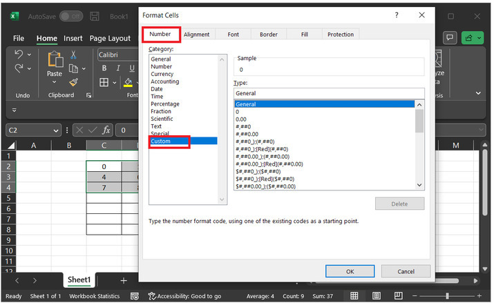
Step 6

In the “Type:” section textbox enters data as “0;-0;;@”, and click on the “OK” button.

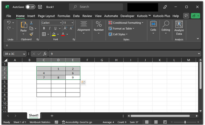
Step 7

Users will be automatically redirected to the original Excel sheet. Users can check that all the cells that contain 0 are empty now. This simply means that all the zero values are hidden normally. In the below given data cell C2, and D3 cells become empty. As these cells' data contain 0 value.

Example 2: To display the zero value from the selected range in Excel

Step 1

This example focuses on displaying the hidden 0 values. For this, consider the above obtained Excel sheet. This Excel sheet contains hidden 0 values.

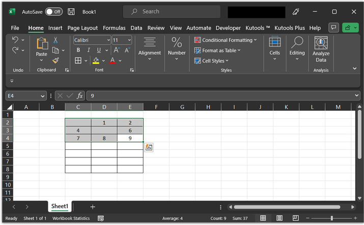
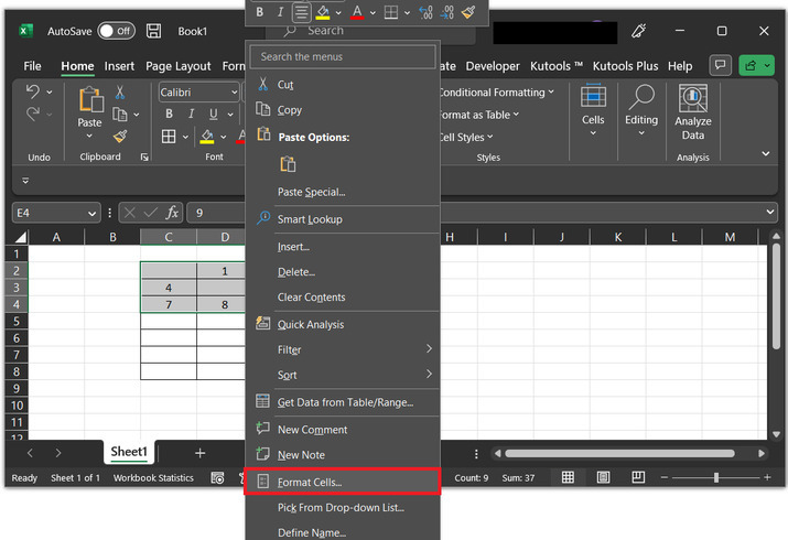
Step 2

Select the available cell range. Once cells are selected, all the cells will be displayed under the grey color cell background. Use right-click with the selected cells, this will display multiple options. Among all the provided options click on the “Format Cells” options.

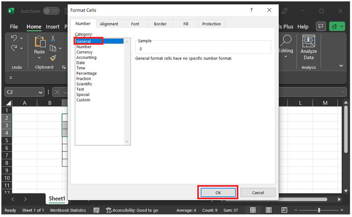
Step 3

This will open the “Format Cells” dialog box. Consider the below image to understand the ongoing processing.

Step 4

After that go select the “General” option and click on the “OK” button.

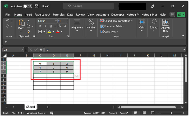
Step 5

This will display all the hidden 0 values again.

Conclusion

In this article user learned both the examples, to hide and unhide the available 0 values. The first example, guide the user to hide the available zeros, while the second method will display the 0 values on the sheet again. Both the provided examples use the option for “Format Cells”.