How to Easily Reverse Selections of Selected Ranges in Excel?

When working with data in Microsoft Excel, choosing individual cells or ranges is a regular activity. However, there may be instances where you need to swiftly invert or reverse your choice for a variety of reasons. Knowing how to reverse your selections can help you save time and effort, whether you wish to exclude specific cells from your selection or just need to deal with the opposite set of cells.

This article will give you simple-to-follow instructions and pointers to help you effectively reverse your selections and streamline your data manipulation process, regardless of your level of Excel proficiency. You will have a thorough understanding of the numerous ways to reverse selections in Excel by the end of this course, enabling you to increase productivity and simplify data manipulation chores. Let's get started and learn the methods that will enable you to quickly reverse choices in Excel!

Easily Reverse Selections of Selected Ranges

Here we will first create a VBA module, then run it and select the range of cells to complete the task. So let us see a simple process to learn how you can easily reverse selections of selected ranges in Excel.

Step 1

Consider an Excel sheet where you have the required data.

First, right-click on the sheet name and select View Code to open the VBA application.

Right-click > View Code.

Step 2

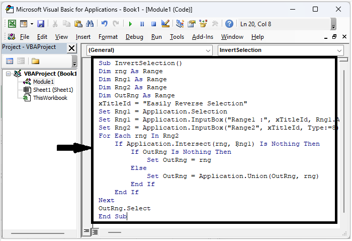
Then click on Insert, select Module, and copy the below code into the text box.

Code

Sub InvertSelection()
Dim rng As Range
Dim Rng1 As Range
Dim Rng2 As Range
Dim OutRng As Range
xTitleId = "Easily Reverse Selection"
Set Rng1 = Application.Selection
Set Rng1 = Application.InputBox("Range1 :", xTitleId, Rng1.Address, Type:=8)
Set Rng2 = Application.InputBox("Range2", xTitleId, Type:=8)
For Each rng In Rng2
   If Application.Intersect(rng, Rng1) Is Nothing Then
      If OutRng Is Nothing Then
         Set OutRng = rng
      Else
         Set OutRng = Application.Union(OutRng, rng)
      End If
   End If
Next
OutRng.Select
End Sub

Insert > Module > Copy.

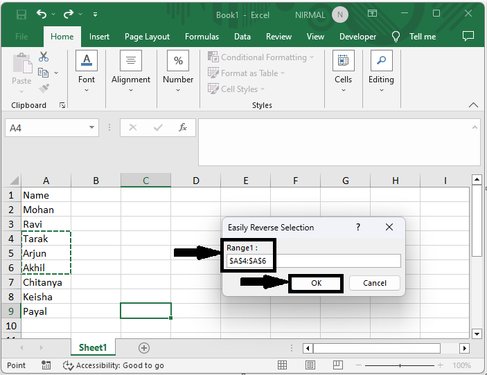
Step 3

Then click F5 to run the Module. Then select the cells that you do not want to select and click OK.

F5 > Select Cells > Ok.

Step 4

Finally, select all the cells in the range and click OK to complete the task.

Select Range > Ok.

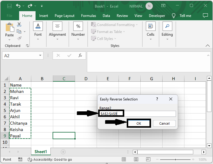
This is how you can reverse the selection of selected ranges in Excel.

Conclusion

In this tutorial, we have used a simple process to show how you can easily reverse selections of selected ranges in Excel to highlight a particular set of data.