
Article Categories
- All Categories
-
 Data Structure
-
 Networking
-
 RDBMS
RDBMS
-
 Operating System
-
 Java
Java
-
 MS Excel
-
 iOS
iOS
-
 HTML
HTML
-
 CSS
CSS
-
 Android
-
 Python
-
 C Programming
-
 C++
C++
-
 C#
C#
-
 MongoDB
-
 MySQL
MySQL
-
 Javascript
-
 PHP
PHP
-
 Economics & Finance
How to Apply Negative VLOOKUP to Return the Value in Left of the Key Field in Excel?
You could have tried to apply the VLOOkUP function to get the values from the right side using the positive numbers, but have you ever tried to get the values from the left side using the VLOOkUP function using the negative values? When we try to use the VLOOKUP for negative values, an error will occur. To solve this problem, we need to apply the VB code to the Excel sheet. Read this tutorial to learn how you can apply negative VLOOKUP to return the value on the left of the key field in Excel.
Apply Negative VLOOKUP to Return the Value on Left of the Key Field
Here we will first add VBA code to the sheet and use the VLOOKUPNEG formula, then use the auto-fill handle to complete the task. Let us see a simple process to understand how we can apply negative VLOOKUP to return the values in the left field of the key field.
Step 1
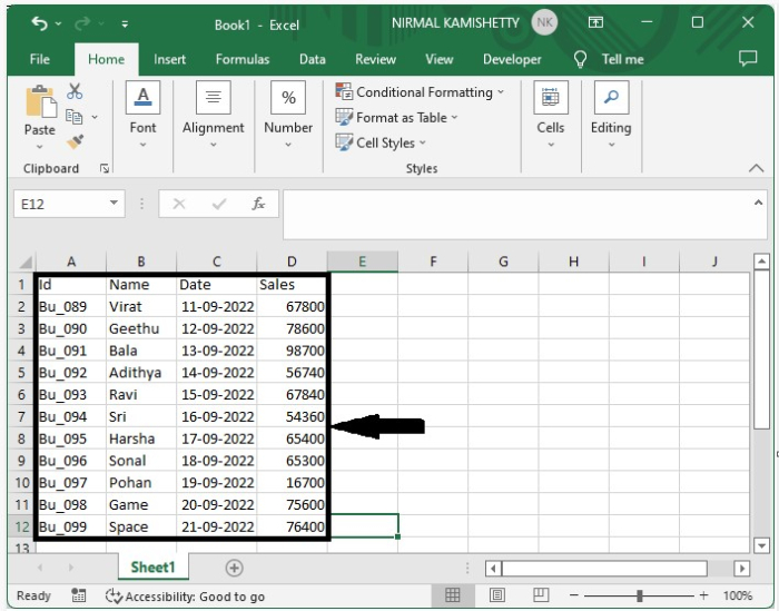
Consider an Excel sheet with data that is similar to the data shown in the image below.
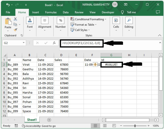
Now when we try to apply the negative VLOOKUP, an error will occur, as shown in the below image.
Step 2
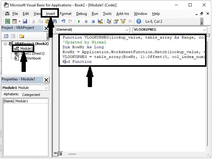
To apply the VBA code, click on the sheet name and select view code to open the VBA application, then click on insert, select module, and type the programme into the text box as shown in the below image.
Program
Function VLOOKUPNEG(lookup_value, table_array As Range, col_index_num As Integer, CloseMatch As Boolean)
   'Updated by Nirmal
   Dim RowNr As Long
   RowNr = Application.WorksheetFunction.Match(lookup_value, table_array.Resize(, 1), CloseMatch)
   VLOOKUPNEG = table_array(RowNr, 1).Offset(0, col_index_num)
End Function
Step 3
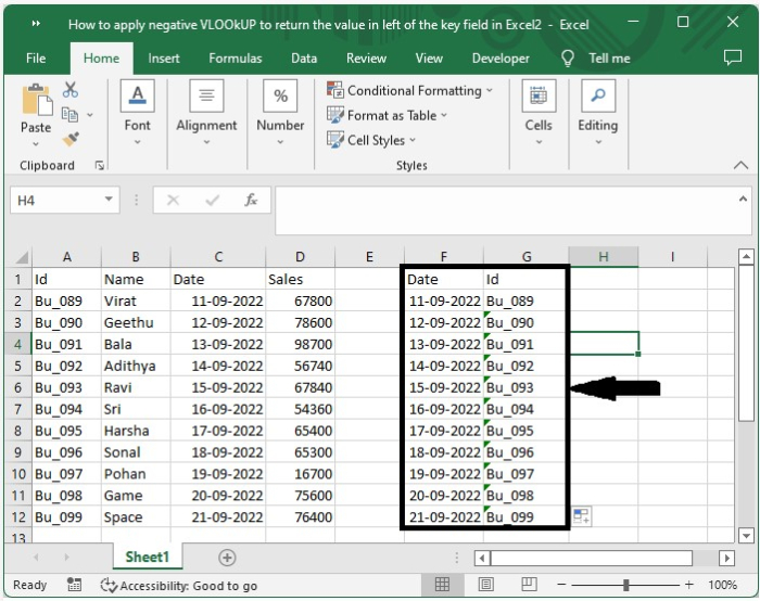
Now save the sheet as VBA enabled, exit the VBA application with the shortcut Alt + Q, and enter the formula =VLOOKUPNEG(F2,C2:C12,-3,0) in the formula box, as shown in the image below.
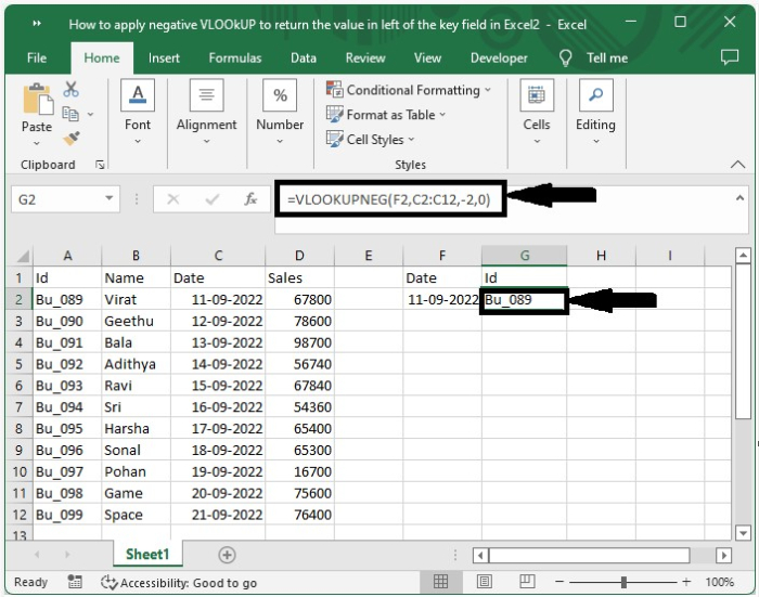
Now to get all the other values, drag from the right corner till all results are filled, and our final output will be similar to the image shown below.
Conclusion
In this tutorial, we used a simple example to demonstrate how we can apply negative VLOOKUP to return the value on the left of the key field in Excel.

2K+ Views
