
Article Categories
- All Categories
-
 Data Structure
-
 Networking
-
 RDBMS
RDBMS
-
 Operating System
-
 Java
Java
-
 MS Excel
-
 iOS
iOS
-
 HTML
HTML
-
 CSS
CSS
-
 Android
-
 Python
-
 C Programming
-
 C++
C++
-
 C#
C#
-
 MongoDB
-
 MySQL
MySQL
-
 Javascript
-
 PHP
PHP
-
 Economics & Finance
How To Do A Case Sensitive Vlookup In Excel?
VLOOKUP is a powerful function that allows you to search for a certain value in a table and obtain information from another column connected with that value. Excel's VLOOKUP function is not case?sensitive by default, which means it handles uppercase and lowercase letters the same. However, there are times when a case?sensitive lookup is required to provide correct results.
In this article, we will go through how to perform a case?sensitive VLOOKUP in Excel step by step. We will go over the functions and strategies required to discover exact matches while taking letter case into account. Mastering this approach will improve your Excel skills and the quality of your results, whether you're working on a data analysis project, managing a database, or simply need to identify specific values in your spreadsheet. So, let's get started and learn how to do a case?sensitive VLOOKUP in Excel!
Do A Case Sensitive Vlookup
Here we will complete the task using a formula. So let us see a simple process to learn how you can do a case?sensitive vlookup in Excel.
Step 1
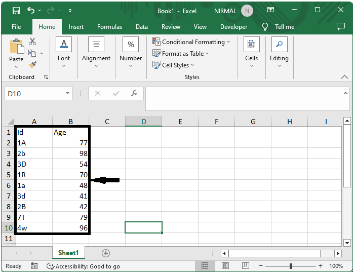
Consider an Excel sheet where the data in the sheet is similar to the below image.
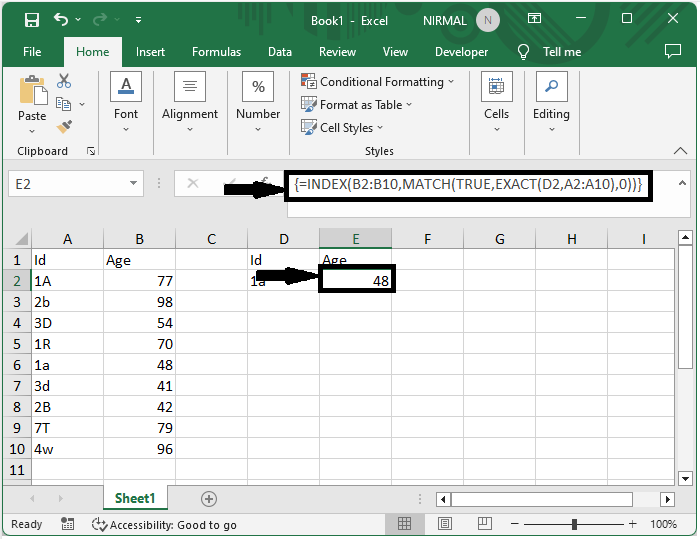
First, click on an empty cell, in our case, cell E2, and enter the formula as =INDEX(B2:B11,MATCH(TRUE,EXACT(D2,A2:A11),0)) and click Ctrl + Shift + Enter to complete the task. In the formula B2:B11, A2:A11 is the range of cells containing data, and D2 is what we are looking for.
Empty cell > Formula > Ctrl + Shift + Enter.
This is how you can do a case?sensitive vlookup in Excel. If you want to apply the Vlookup without the case sensitive you can directly use the formula with VLOOKUP key word.
Conclusion
In this tutorial, we have used a simple example to demonstrate how you can do a case?sensitive vlookup in Excel to highlight a particular set of data.

1K+ Views
