
Article Categories
- All Categories
-
 Data Structure
-
 Networking
-
 RDBMS
RDBMS
-
 Operating System
-
 Java
Java
-
 MS Excel
-
 iOS
iOS
-
 HTML
HTML
-
 CSS
CSS
-
 Android
-
 Python
-
 C Programming
-
 C++
C++
-
 C#
C#
-
 MongoDB
-
 MySQL
MySQL
-
 Javascript
-
 PHP
PHP
-
 Economics & Finance
How to Alternate Row Colour Based on Group in Excel?
As we all know that we can change the colour of alternate rows with different colours very easy in excel but have you ever wondered can alternate row colour based on the condition the condition can be anything. We will try to choose the colour for the row based on a single condition. We can achieve this by just following this simple process to alternate row colour based on group in excel
Let us see a simple process to alternate row colour in Excel based on group.
Step 1
Let us assume a situation where we have a data where there are multiple items in a column of data and we are altering the row colour based on group on the condition of similar items. In order to do that, we need to find the duplicate items in the list and assign a number to them and enter "B2" element as "0".
To do that, click the empty cell which is in our case "B2" and enter formula as
"=IF (A2=A1, B1, B1+1)"
Then click on enter to get the first result as shown in the figure below ?
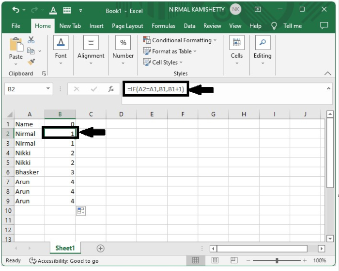
Now drag down for the right corner of the first result to get the results. Then all the items are grouped based on number from 1-4.
Step 2
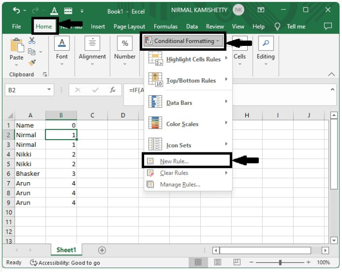
Now select the data and then click "conditional formatting" under "Home" on the "Quick Access" toolbar and select "New Rule" to open a new pop-up.
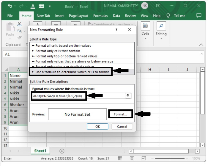
In the new pop-up window, select "use a formula to determine the format" and enter the formula as
"=AND(LEN($A2)>0, MOD($B2,2) =0)"
And click "Format" to open a new pop-up.
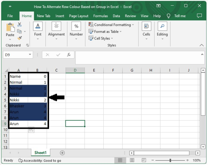
Step 3
In the new pop-up, click "Fill" and select a colour and then click "ok" to complete the process.
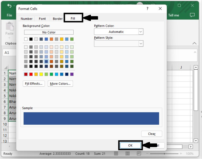
Our final output will look like the screenshot below ?

885 Views
