How To Directly Jump To Next Duplicate Cell In Excel?

Duplicate value management is a regular chore when working with huge datasets or lists. Excel offers a number of helpful features to make navigating and working with your data easier. This course will concentrate on one particular scenario− finding and moving on to the subsequent instance of a duplicate value within a column. We will look at an easy way to go right to the next duplicate cell instead of having to manually scroll through your spreadsheet to find it.

By following the guidelines in this tutorial, you may speed up and streamline your process while working with duplicate data in Excel. Let's get going and see how to rapidly navigate to the following duplicate cell in Excel!

Directly Jump To Next Duplicate Cell

Here, we can complete the task by following the simple procedure mentioned in this tutorial. So let us see a simple process to see how you can directly jump to the next duplicate cell in Excel.

Step 1

Consider an Excel sheet where you have a list of items with duplicates, similar to the below image.

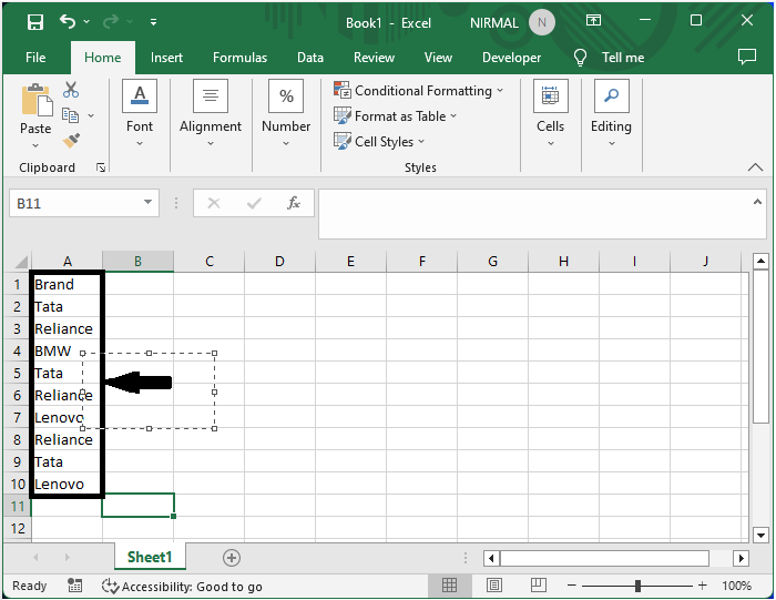
First, click on an empty cell and enter the formula as =MATCH(A2,A3:$A10,0) then click enter and drag down using the autofill handle.

Empty cell > Formula > Enter > Drag.

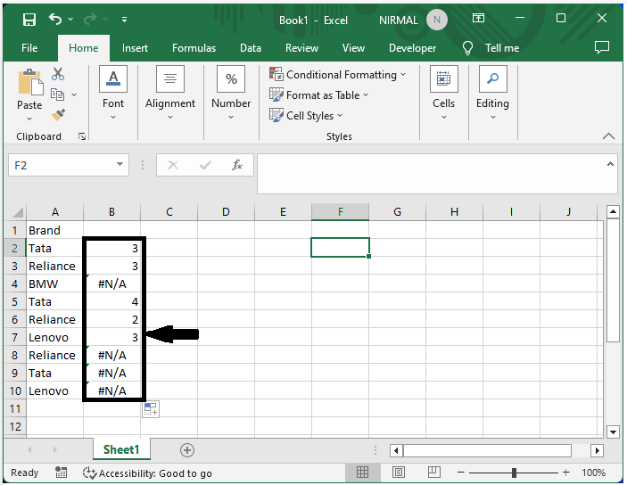
Step 2

Now again, click on an empty cell, enter the formula as =IFERROR(B2,0) and click enter, and drag down using the autofill handle.

Empty cell > Formula > Enter > Drag.

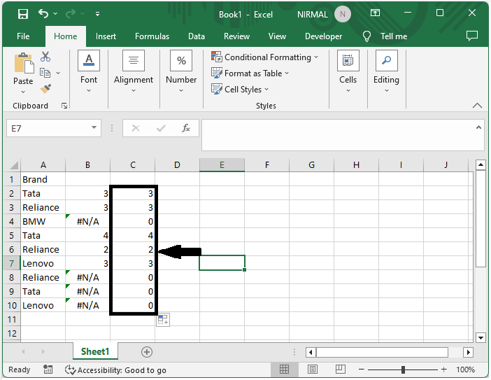
Step 3

Then click on another empty cell and enter the formula as =ROW(A2), click enter, and drag down using the autofill handle.

Empty cell > Formula > Enter > Drag.

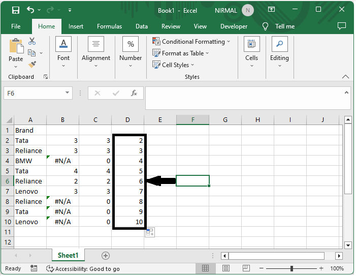
Step 4

Then in cell E2, enter the formula as =C2+D2 and click enter, then drag down using the autofill handle.

Empty cell > Formula > Enter > Drag.

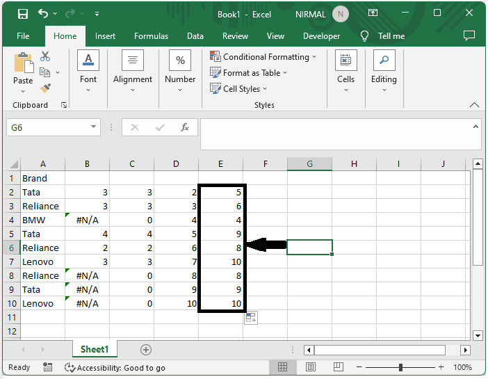
Step 5

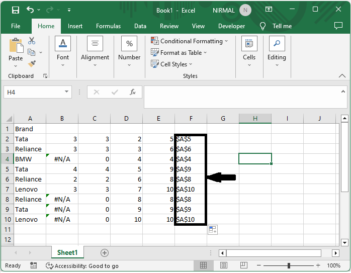
Then in cell F2, enter the formula as =ADDRESS(E2,1) and click enter, and drag down using the autofill handle.

Empty cell > Formula > Enter > Drag.

Step 6

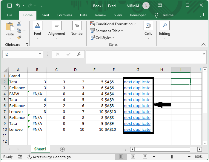
Then in cell G2, enter the formula as =HYPERLINK("#"&F2,"next duplicate"), click enter, and drag down using the autofill handle to complete the task.

Empty cell > Formula > Enter > Drag.

Conclusion

In this tutorial, we have used a simple example to demonstrate how you can directly jump to the next duplicate cell in Excel to highlight a particular set of data.