
Article Categories
- All Categories
-
 Data Structure
-
 Networking
-
 RDBMS
RDBMS
-
 Operating System
-
 Java
Java
-
 MS Excel
-
 iOS
iOS
-
 HTML
HTML
-
 CSS
CSS
-
 Android
-
 Python
-
 C Programming
-
 C++
C++
-
 C#
C#
-
 MongoDB
-
 MySQL
MySQL
-
 Javascript
-
 PHP
PHP
-
 Economics & Finance
How to rank duplicate values in Excel?
To ascertain a value's rank or placement inside a list of numbers in Excel, use the "RANK" function. The rank shows where a value stands in relation to other values in the dataset.
The goal of rating duplicate values in Excel is to give each duplicate value a ranking or position depending on their magnitude or order. This method is useful if users have a list of data with duplicate values and want to know where each duplicate value is in relation to the others in the dataset. Charts and graphs can be used to visualize ranked duplicate values, which improves communication of the data distribution. Additionally, they make data reporting simpler, which facilitates information presentation to stakeholders.
Example 1: To Rank Duplicate Values in Excel
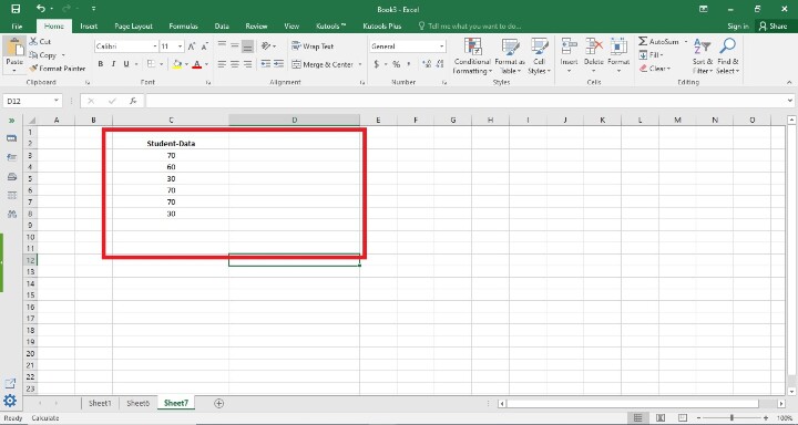
Step 1
In the first step, users create one column in the worksheet i.e. Student-Data. Following is the screenshot of this step.
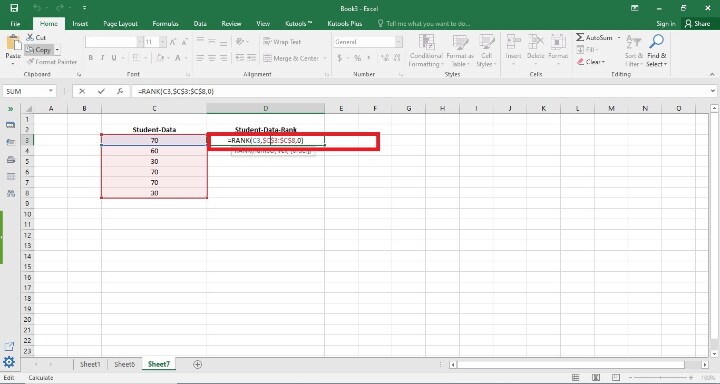
Step 2
In this step, users created one more column in cell D2 i.e. Student-Data-Rank . After that, they apply the formula =Rank(C3,$C$3:$C$8,0). Following is the screenshot of this step.
Explanation
Rank(C3,$C$3:$C$8,0) Excel's "RANK" function requires three arguments: the value users wish to rank, a reference to the cell range containing the data, and an optional argument specifying the ranking order (1 for ascending, 0 for descending). By taking into account duplicate values and ranking the values in descending order (biggest to smallest), this formula uses Excel's "RANK" function to calculate the rank of the value in cell C3 within the range C3:C8.
Excel will rank the value in cell C3 within the range C3:C8 after users enter this formula and display the results. Remember that duplicate values will be given the same rank and will cause the next rank to be skipped if there are any in the range.
In the above formula, they have taken 3 arguments that are given below
"number" means the item in cell C3 that users want to rank.
The reference "ref" refers to the range of cells that contain the data they want to rank. $C$3:$C$8.
The optional argument "order" defines the ranking order. Since 0 denotes descending order, the largest value will be at the bottom of the list.
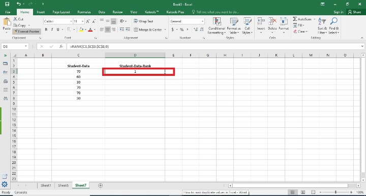
Step 3
In this step, users enter the D3 cell. In this step, users have seen the rank there. Following is the screenshot of this step.
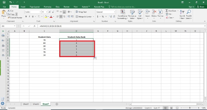
Step 4
In this step, users find the remaining result of Student-Data-Rank . Users may accomplish this by dragging the fill handle to the final cell where the user wants the rankings to appear (it's a tiny square in the bottom-right area of that row). Following is the screenshot of this step.
Conclusion
Users can quickly find and contrast duplicate values in a dataset by ranking duplicates. It gives a visual illustration of the positions of duplicate numbers in relation to one another, making it simpler to identify patterns or trends.
All of the instructions are clear, trustworthy, and brief. By using the instructions in the aforementioned stages, the user can give duplicate ranks to the corresponding student data.

5K+ Views
