How to highlight the last duplicate row/cell in Excel?

In the article, the users are going to highlight the last duplicate row in Microsoft Excel. There are several features in the Excel sheet including Ku-tools, Filter, and Auto Fill tab that the users have to fill any type of color according to their needs. The users can use the formula for counting the numbers in the row. The users can use select the range in which they want to fill the color in any cell. The two examples are depicted in this article, example 1 uses the concept of Filter option and example 2 illustrates the Kutools to highlight the last duplicate row/cell in Excel.

To highlight the last duplicate row/cell in Excel

By using the Filter option

Step 1

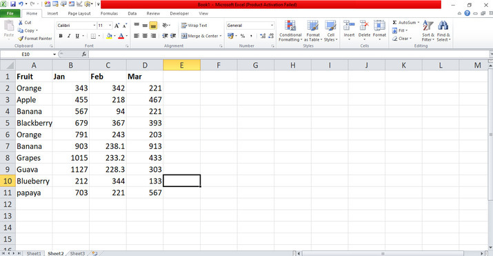
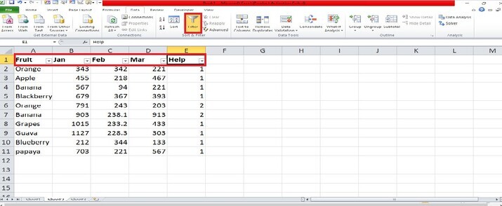
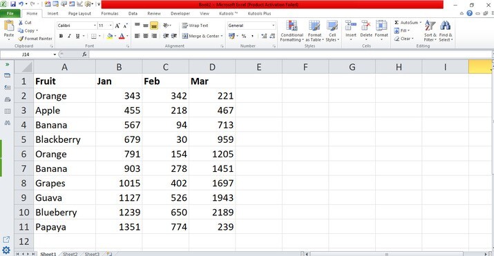
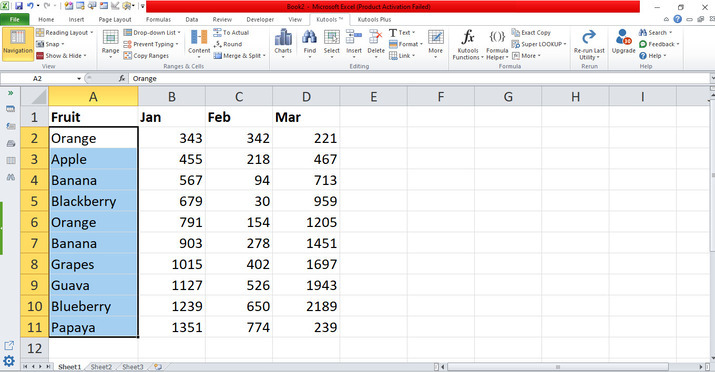
Deliberate the Excel sheet with the data. First, open the Excel sheet and create the data one by one. In this sheet, type any type the data like Fruit, and the months like January, February, and March fields. The users have to count duplicate rows which the users need to highlight the cells in the given list as shown below.

Step 2

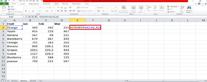
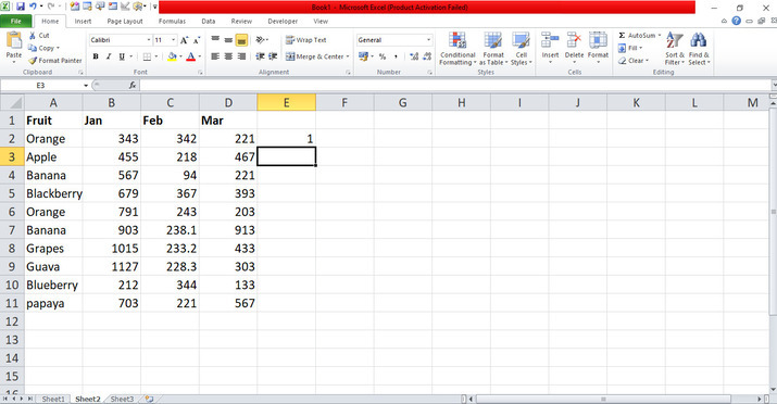
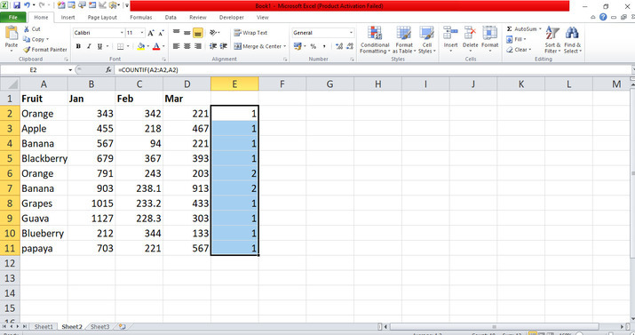
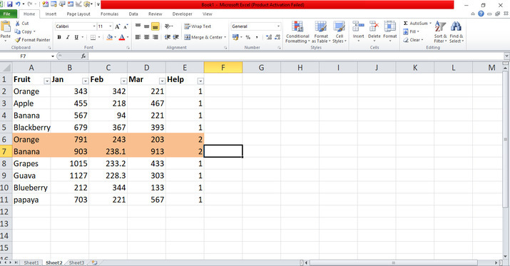
In the excel sheet, the created data is displayed. Place the cursor in the empty cell E2 and enter the formula =COUNTIF(A2:A2,A2) that counts the number of the rows. Now, select the row and drag it by last cell to fill the values one by one as shown below.

Step 3

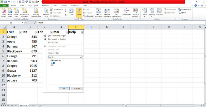
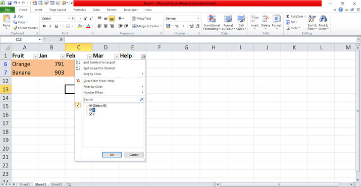
Select the Help row to filter the sorted values. In the ribbon, there are many tabs included in the top corner. Place the cursor in the Data tab and click on the tab that has many options included. On the Data tab, place the cursor on the Filter tab which has included in the Sort & Filter group. On this tab, click on the Filter tab that will visible the drop-down menu in all rows as well as the Help row. After selecting the row in the sheet, click on the drop-down menu that will open the dialog box. In the dialog box, deselect the count 1 that will only mention duplicate values as shown below.

Step 4

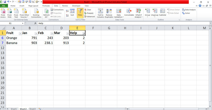
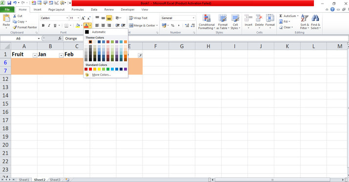
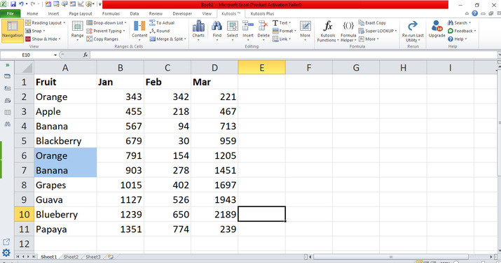
In the sheet, the only duplicate values included are the Orange and Banana rows. Now, the users need to highlight the duplicate rows. In the ribbon, there are many tabs included in the top corner. Place the cursor in the Home tab and click on the tab that has many options included. Select all the rows, place the cursor, and click on the Fill Color tab that has many colors. Choose any type of color to highlight the duplicate values as shown below.

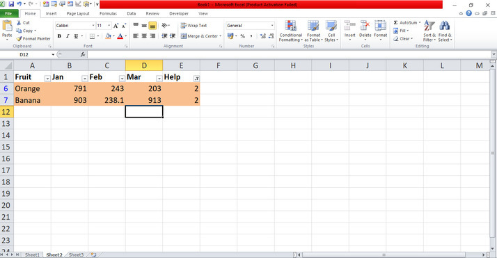
Step 5

In the sheet, the users need to view all the rows that have duplicate and non-duplicate values. Place the cursor in the Help row and select the count 1 to visible all the rows like this.

By using Kutools tab

Step 1

Deliberate the excel sheet with the data. First, open the excel sheet and create the data one by one. In this sheet, type any type the data like Fruit, and the months like January, February and March fields. The users have to count duplicate rows which the users need to highlight the cells in the given list as shown below.

Step 2

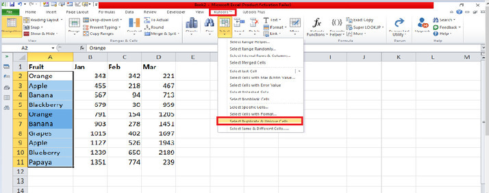
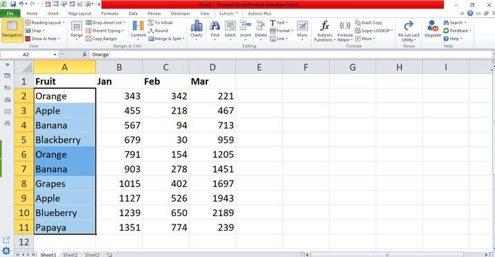
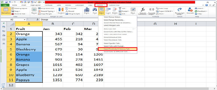
In the Excel sheet, the created data is displayed. Place the cursor in cell A2 and select all the cells to A11 that will highlight duplicate rows. After selecting the column, place the cursor in the Ku-tools tab and click on the tab that has many options included. On the Ku-tools tab, place the cursor on the Select tab which has included in the Editing group. On this tab, click on the Select tab which has many options. Click on the drop-down menu and click on the Select duplicate & unique cells tab that will open the dialog box.

Step 3

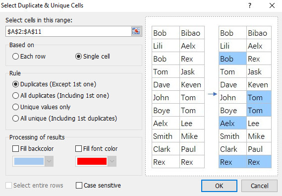
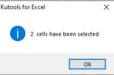
In the dialog box, enable the option Duplicates which will enable the Fill back-color box, and click on the ok button that will highlight only duplicate rows as shown below.

Step 4

In the Excel sheet, the updated data is displayed. Place the cursor in cell A2 and select all the cells to A11 that will highlight duplicate rows. After selecting the column, place the cursor in the Ku-tools tab and click on the tab that has many options included. On the Ku-tools tab, place the cursor on the Select tab which has included in the Editing group. On this tab, click on the Select tab which has many options. Click on the drop-down menu and click on the Select duplicate & unique cells tab that will open the dialog box.

Step 5

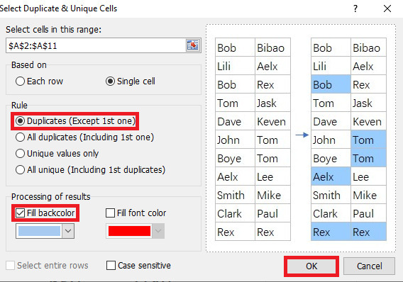
In the dialog box, enable the option Duplicates which will enable the Fill back-color box, and click on the ok button that will highlight only duplicate rows as shown below.

The users utilized an easy instance to display how can highlight the duplicate rows with the Ku-tools tab and using a formula. The users used the necessary tabs which are included in the ribbon. The users have to practice the essential options from the ribbon and modify the data according to their needs.