How to hide duplicate records in columns in Excel?

Duplicate data is information that has been entered into numerous Excel cells, sheets, or other objects. Data can be repeated across several rows, columns, and pages. Duplicate data increases data complexity and ambiguities. Therefore, it is suggested that users should not repeat the data until it is required very badly. One might occasionally need to retain the unique values for columns in Excel while hiding all duplicates.

In this article, we'll demonstrate how to use Excel to hide all duplicates, including/excluding the first one. This article briefs two approaches. The first approach uses conditional formatting to hide duplicate values. While the second method is based on the process of using the kutool. Hiding duplicate data values will cause pros and cons actions. In good terms, it can make data easy, simple, and redundancy-proof. While in the negative aspect, the data will become uneven.

Example 1: To hide the duplicate records in columns by using the conditional formatting option in Excel

Step 1

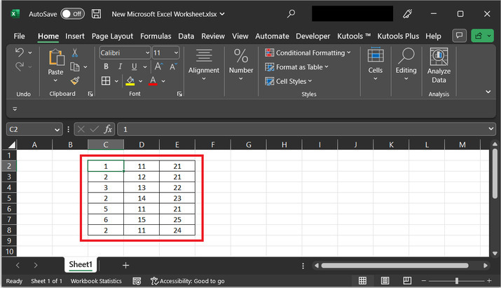
To understand the process of hiding the data, by using the conditional formatting option. Consider the below given 21 elements. this grid contains some duplicate value. In this example, will try to remove the duplicate records from the columns in excel.

Step 2

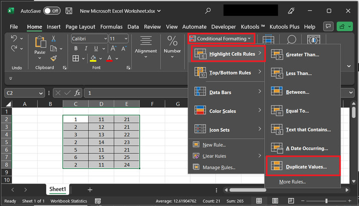
Now click on the “Home” Tab. Click on the “Conditional Formatting” option, under the Styles group. Further, select the option “Duplicate values..”. Consider the below-depicted image for proper reference −

Step 3

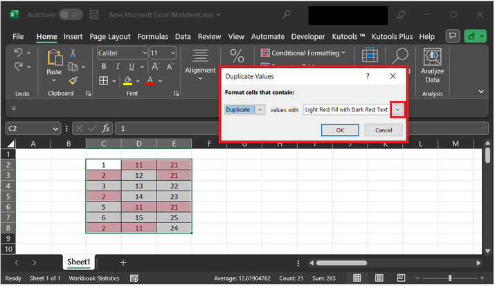
The above step will open a “Duplicate Values” dialog box, and then select the drop-down arrow, as shown below in the image −

Step 4

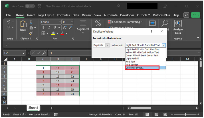
The drop-down menu will display multiple options, as specified in the image. Finally, select the option “Custom Format”.

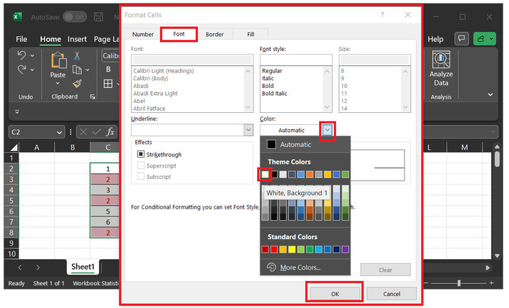
Step 5

The above step will open a “Format Cells” dialog box. This dialog box, contains multiple tabs, such as number, font, and many others. Select the “Font” tab, and then under the color section click on the drop-down menu. From the appeared list of color select the “white” color. Finally, click on “OK” button twice in the appeared dialog box.

Step 6

The above step will remove all the duplicate values and you may also select the boundary of the table in grid form. Consider the below-given image for reference.

Example 2: To hide the duplicate records in columns by using the kutool option in Excel

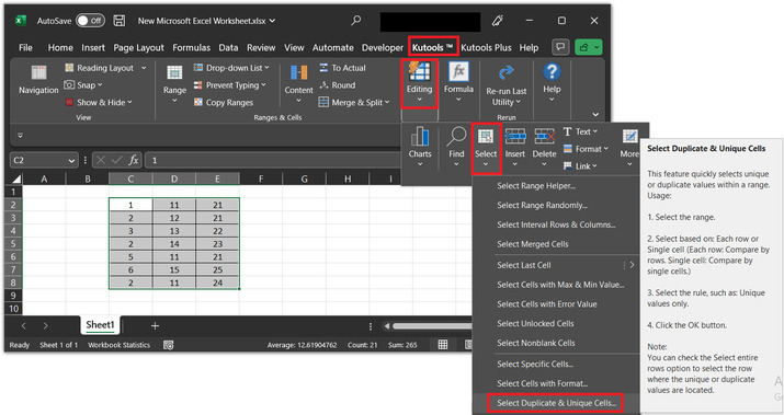
Step 1

Again, consider the same worksheet. To use the Kutool tab, click on the “Editing” tab, under the editing option, and choose the “Select” option. Further, click on “Select Duplicate & Unique Cells”.

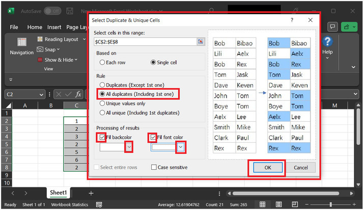
Step 2

The above step will display a “Select Duplicate & Unique Cells” dialog box. In the appeared dialog box, under the rule label, select the option “All duplicates (including the 1st one)” In the processing of result label, tick the option for “Fill backcolor”, and select the white color. Similarly, tick the option for “Fill font color”. Click on the drop-down menu, and choose the “white” color.

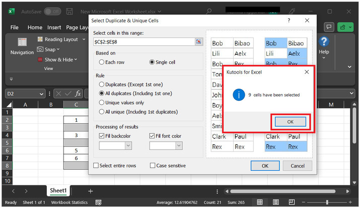
Step 3

Click on the “OK” button. this will display the count of cells with duplicate values within the “Kutools for Excel” dialog box. Finally, press the “OK” button.

Step 4

Consider the below-given snapshot for output.

Conclusion

This article user will understand the process of using Conditional Formatting and Kutools for Excel to hide the duplicate record values of the column data. By using both methods users can easily hide the duplicate records in columns. Both the provided methods are efficient and capable of processing the required data.