- Excel Functions - Home
- Compatibility Functions
- Compatibility Functions
- BETADIST Function
- BETAINV Function
- BINOMDIST Function
- CEILING Function
- CHIDIST Function
- CHIINV Function
- CHITEST Function
- CONFIDENCE Function
- COVAR Function
- CRITBINOM Function
- EXPONDIST Function
- FDIST Function
- FINV Function
- FLOOR Function
- FTEST Function
- GAMMADIST Function
- GAMMAINV Function
- HYPGEOMDIST Function
- LOGINV Function
- LOGNORMDIST Function
- MODE Function
- NEGBINOMDIST Function
- NORMDIST Function
- NORMINV Function
- NORMSDIST Function
- NORMSINV Function
- PERCENTILE Function
- PERCENTRANK Function
- POISSON Function
- QUARTILE Function
- RANK Function
- STDEV Function
- STDEVP Function
- TDIST Function
- TINV Function
- TTEST Function
- VAR Function
- VARP Function
- WEIBULL Function
- ZTEST Function
- Logical Functions
- Logical Functions
- AND Function
- FALSE Function
- IF Function
- IFERROR Function
- IFNA Function
- IFS Function
- NOT Function
- OR Function
- SWITCH Function
- TRUE Function
- XOR Function
- Text Functions
- Text Functions
- ARRAYTOTEXT Function
- BAHTTEXT Function
- CHAR Function
- CLEAN Function
- CODE Function
- CONCAT Function
- CONCATENATE Function
- DBCS Function
- DOLLAR Function
- Exact Function
- FIND Function
- FINDB Function
- FIXED Function
- LEFT Function
- LEFTB Function
- LEN Function
- LENB Function
- LOWER Function
- MID Function
- MIDB Function
- NUMBERVALUE Function
- PHONETIC Function
- PROPER Function
- REPLACE Function
- REPLACEB Function
- REPT Function
- RIGHT Function
- RIGHTB Function
- SEARCH Function
- SEARCHB Function
- SUBSTITUTE Function
- T Function
- TEXT Function
- TEXTAFTER Function
- TEXTBEFORE Function
- TEXTJOIN Function
- TEXTSPLIT Function
- TRIM Function
- UNICHAR Function
- UNICODE Function
- UPPER Function
- VALUE Function
- VALUETOTEXT Function
- Date & Time Functions
- Date & Time Functions
- DATE Function
- DATEDIF Function
- DATEVALUE Function
- DAY Function
- DAYS Function
- DAYS360 Function
- EDATE Function
- EOMONTH Function
- HOUR Function
- ISOWEEKNUM Function
- MINUTE Function
- MONTH Function
- NETWORKDAYS Function
- NETWORKDAYS.INTL Function
- NOW Function
- SECOND Function
- TIME Function
- TIMEVALUE Function
- TODAY Function
- WEEKDAY Function
- WEEKNUM Function
- WORKDAY Function
- WORKDAY.INTL Function
- YEAR Function
- YEARFRAC Function
- Cube Functions
- Cube Functions
- CUBEKPIMEMBER Function
- CUBEMEMBER Function
- CUBEMEMBERPROPERTY Function
- CUBERANKEDMEMBER Function
- CUBESET Function
- CUBESETCOUNT Function
- CUBEVALUE Function
- Math Functions
- Math Functions
- ABS Function
- AGGREGATE Function
- ARABIC Function
- BASE Function
- CEILING.MATH Function
- COMBIN Function
- COMBINA Function
- DECIMAL Function
- DEGREES Function
- EVEN Function
- EXP Function
- FACT Function
- FACTDOUBLE Function
- FLOOR.MATH Function
- GCD Function
- INT Function
- LCM Function
- LN Function
- LOG Function
- LOG10 Function
- MDETERM Function
- MINVERSE Function
- MMULT Function
- MOD Function
- MROUND Function
- MULTINOMIAL Function
- MUNIT Function
- ODD Function
- PI Function
- POWER Function
- PRODUCT Function
- QUOTIENT Function
- RADIANS Function
- RAND Function
- RANDBETWEEN Function
- ROMAN Function
- ROUND Function
- ROUNDDOWN Function
- ROUNDUP Function
- SERIESSUM Function
- SIGN Function
- SQRT Function
- SQRTPI Function
- SUBTOTAL Function
- SUM Function
- SUMIF Function
- SUMIFS Function
- SUMPRODUCT Function
- SUMSQ Function
- SUMX2MY2 Function
- SUMX2PY2 Function
- SUMXMY2 Function
- TRUNC Function
- Trigonometric Functions
- Trigonometric Functions
- ACOS
- ACOSH Function
- ACOT Function
- ACOTH Function
- ASIN Function
- ASINH Function
- ATAN Function
- ATAN2 Function
- ATANH Function
- COS Function
- COSH Function
- COT Function
- COTH Function
- CSC Function
- CSCH Function
- SEC Function
- SECH Function
- SIN Function
- SINH Function
- TAN Function
- TANH Function
- Database Functions
- Database Functions
- DAVERAGE
- DCOUNT
- DCOUNTA
- DGET
- DMAX
- DMIN
- DPRODUCT
- DSTDEV
- DSTDEVP
- DSUM
- DVAR
- DVARP
- Dynamic Array Functions
- Dynamic Array Functions
- FILTER Function
- RANDARRAY Function
- SEQUENCE Function
- SORT Function
- SORTBY Function
- UNIQUE Function
- XLOOKUP Function
- XMATCH Function
- Engineering Functions
- Engineering Functions
- BESSELI Function
- BESSELJ Function
- BESSELK Function
- BESSELY Function
- BIN2DEC Function
- BIN2HEX Function
- BIN2OCT Function
- BITAND Function
- BITLSHIFT Function
- BITOR Function
- BITRSHIFT Function
- BITXOR Function
- COMPLEX Function
- CONVERT Function
- DEC2BIN Function
- DEC2HEX Function
- DEC2OCT Function
- DELTA Function
- ERF Function
- ERF.PRECISE Function
- ERFC Function
- ERFC.PRECISE Function
- GESTEP Function
- HEX2BIN Function
- HEX2DEC Function
- HEX2OCT Function
- IMABS Function
- IMAGINARY Function
- IMARGUMENT Function
- IMCONJUGATE Function
- IMCOS Function
- IMCOSH Function
- IMCOT Function
- IMCSC Function
- IMCSCH Function
- IMDIV Function
- IMEXP Function
- IMLN Function
- IMLOG2 Function
- IMLOG10 Function
- IMPOWER Function
- IMPRODUCT Function
- IMREAL Function
- IMSEC Function
- IMSECH Function
- IMSIN Function
- IMSINH Function
- IMSQRT Function
- IMSUB Function
- IMSUM Function
- IMTAN Function
- OCT2BIN Function
- OCT2DEC Function
- OCT2HEX Function
- Financial Functions
- Financial Functions
- ACCRINT Function
- ACCRINTM Function
- AMORDEGRC Function
- AMORLINC Function
- COUPDAYBS Function
- COUPDAYS Function
- COUPDAYSNC Function
- COUPNCD Function
- COUPNUM Function
- COUPPCD Function
- CUMIPMT Function
- CUMPRINC Function
- DB Function
- DDB Function
- DISC Function
- DOLLARDE Function
- DOLLARFR Function
- DURATION Function
- EFFECT Function
- FV Function
- FVSCHEDULE Function
- INTRATE Function
- IPMT Function
- IRR Function
- ISPMT Function
- MDURATION Function
- MIRR Function
- NOMINAL Function
- NPER Function
- NPV Function
- ODDFPRICE Function
- ODDFYIELD Function
- ODDLPRICE Function
- ODDLYIELD Function
- PDURATION Function
- PMT Function
- PPMT Function
- PRICE Function
- PRICEDISC Function
- PRICEMAT Function
- PV Function
- RATE Function
- RECEIVED Function
- RRI Function
- SLN Function
- SYD Function
- TBILLEQ Function
- TBILLPRICE Function
- TBILLYIELD Function
- VDB Function
- XIRR Function
- XNPV Function
- YIELD Function
- YIELDDISC Function
- YIELDMAT Function
- Information Functions
- Information Functions
- CELL Function
- ERROR.TYPE Function
- INFO Function
- ISBLANK Function
- ISERR Function
- ISERROR Function
- ISEVEN Function
- ISFORMULA Function
- ISLOGICAL Function
- ISNA Function
- ISNONTEXT Function
- ISNUMBER Function
- ISODD Function
- ISREF Function
- ISTEXT Function
- N Function
- NA Function
- SHEET Function
- SHEETS Function
- TYPE Function
- Lookup & Reference Functions
- Lookup & Reference Functions
- ADDRESS Function
- AREAS Function
- CHOOSE Function
- COLUMN Function
- COLUMNS Function
- FORMULATEXT Function
- GETPIVOTDATA Function
- HLOOKUP Function
- HYPERLINK Function
- INDEX Function
- INDIRECT Function
- LOOKUP Function
- MATCH Function
- OFFSET Function
- ROW Function
- ROWS Function
- RTD Function
- TRANSPOSE Function
- VLOOKUP Function
- Statistical Functions
- Statistical Functions
- AVEDEV Function
- AVERAGE Function
- AVERAGEA Function
- AVERAGEIF Function
- AVERAGEIFS Function
- BETA.DIST Function
- BETA.INV Function
- BINOM.DIST Function
- BINOM.DIST.RANGE Function
- BINOM.INV Function
- CHISQ.DIST Function
- CHISQ.DIST.RT Function
- CHISQ.INV Function
- CHISQ.INV.RT Function
- CHISQ.TEST Function
- CONFIDENCE.NORM Function
- CONFIDENCE.T Function
- CORREL Function
- COUNT Function
- COUNTA Function
- COUNTBLANK Function
- COUNTIF Function
- COUNTIFS Function
- COVARIANCE.P Function
- COVARIANCE.S Function
- DEVSQ Function
- EXPON.DIST Function
- F.DIST Function
- F.DIST.RT Function
- F.INV Function
- F.INV.RT Function
- F.TEST Function
- FISHER Function
- FISHERINV Function
- FORECAST Function
- FORECAST.ETS Function
- FORECAST.ETS.CONFINT Function
- FORECAST.ETS.SEASONALITY Function
- FORECAST.ETS.STAT Function
- FORECAST.LINEAR Function
- FREQUENCY Function
- GAMMA Function
- GAMMA.DIST Function
- GAMMA.INV Function
- GAMMALN Function
- GAMMALN.PRECISE Function
- GAUSS Function
- GEOMEAN
- GROWTH
- HARMEAN
- HYPGEOM.DIST
- INTERCEPT Function
- KURT Function
- LARGE Function
- LINEST Function
- LOGEST Function
- LOGNORM.DIST Function
- LOGNORM.INV Function
- MAX Function
- MAXA Function
- MAXIFS Function
- MEDIAN Function
- MIN Function
- MINA Function
- MINIFS Function
- MODE.MULT Function
- MODE.SNGL Function
- NEGBINOM.DIST Function
- NORM.DIST Function
- NORM.INV Function
- NORM.S.DIST Function
- NORM.S.INV Function
- PEARSON Function
- PERCENTILE.EXC
- PERCENTILE.INC
- PERCENTRANK.EXC
- PERCENTRANK.INC
- PERMUT
- PERMUTATIONA
- PHI
- POISSON.DIST
- PROB
- QUARTILE.EXC
- QUARTILE.INC
- RANK.AVG
- RANK.EQ
- RSQ
- SKEW
- SKEW.P
- SLOPE
- SMALL
- STANDARDIZE
- STDEV.P
- STDEV.S
- STDEVA
- STDEVPA
- STEYX
- T.DIST
- T.DIST.2T
- T.DIST.RT
- T.INV
- T.INV.2T
- T.TEST
- TREND
- TRIMMEAN Function
- VAR.P Function
- VAR.S Function
- VARA Function
- VARPA Function
- WEIBULL.DIST Function
- Z.TEST Function
- Web Functions
- Web Functions
- ENCODEURL Function
- FILTERXML Function
- WEBSERVICE Function
Excel - TEXTAFTER Function
TEXTAFTER Function
The Excel TEXTAFTER function retrieves the text after matching the delimiter/character/text either from the front or rear side of the text string. The TEXTAFTER function is not available in the older version of Microsoft Excel and is contrary to the TEXTBEFORE function. By default, this function is case-sensitive. You can set the match_mode argument to 1 for case insensitive. For example, you can extract the extensions of multiple image files on the laptop.
Compatibility
This advanced Excel function is compatible with the following versions of MS-Excel −
- Excel for Microsoft 365
- Excel for Microsoft 365 for Mac
- Excel for the web
Syntax
The syntax of the TEXTAFTER function is as follows −
=TEXTAFTER(text,delimiter,[instance_num], [match_mode],
   [match_end], [if_not_found])
Arguments
You can use the following arguments with the TEXTAFTER function −
| Argument | Description | Required / Optional |
|---|---|---|
| Text | It specifies the text string to fetch the specific text. | Required |
| Delimiter | A specific text that acts as a point is presented in the string. After that point, you can retrieve the text. | Required |
| instance_num | It indicates the delimiters instance to retrieve the resulting text. By default, its value is 1. If its value is negative, text searching is from the rear. | Optional |
| match_mode | This argument contains a binary value of 0 or 1. By default, 0 is used for case sensitive. Otherwise, write 1 for case insensitive. | Optional |
| match_end | Its value can be 0 or 1, 0 for no match to end and 1 for match to end. By default, 0 is used. It considers the texts rear as a delimiter. | Optional |
| If_not_found | The specific text message will be retrieved if no text match is found. | Optional |
Points to Remember
- If the delimiter is not matched in the text string, the TEXTAFTER function will retrieve the #N/A error.
- If the instance_num is larger than the text string or equivalent to zero, then the TEXTAFTER function will retrieve the #VALUE! error.
- The TEXTAFTER function will display a null value if the cell references empty string values.
Examples of TEXTAFTER Function
Lets elaborate with a few exciting examples of the TEXTAFTER function.
Example 1
The TEXTAFTER function in Excel is a text manipulation function that allows you to extract the portion of a string that appears after a specified delimiter.
Solution
Step 1 − Assume the sample dataset consists of two columns named Product ID and Serial Number.

Step 2 − Write the formula =TEXTAFTER(A3,"-") in the B3 cell and press the Enter.
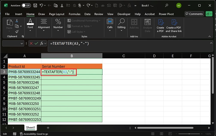
The TEXTAFTER function will return the only serial number just after the -delimiter.

Step 3 − Similarly, you can retrieve the serial numbers of the other remaining cells by dragging the + sign at the bottom right corner of the B3 cell to the B12 cell.

Example 2: Using Multiple Delimiters
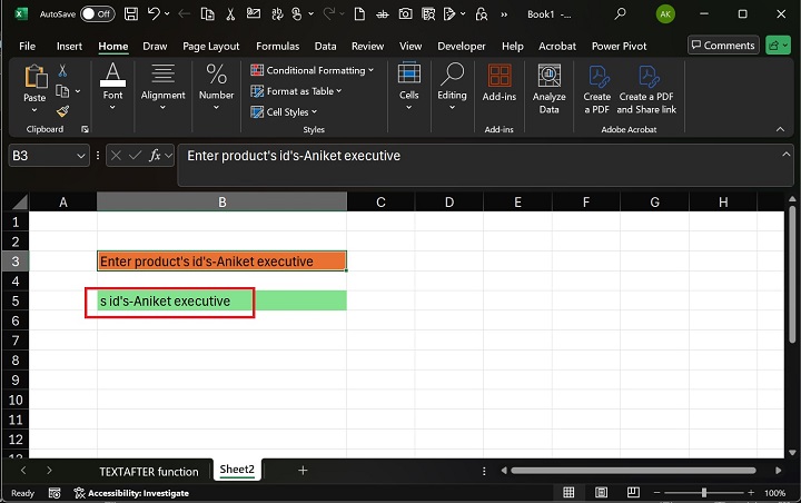
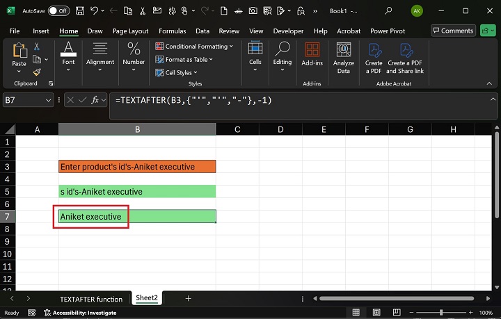
Lets say the text string contains various delimiters. Then, in this case, you can use the array and specify all delimiters separated by the commas in the second argument. Enter the formula =TEXTAFTER(B3,{"'","'","-"}) in the B5 cell and press the Enter tab.
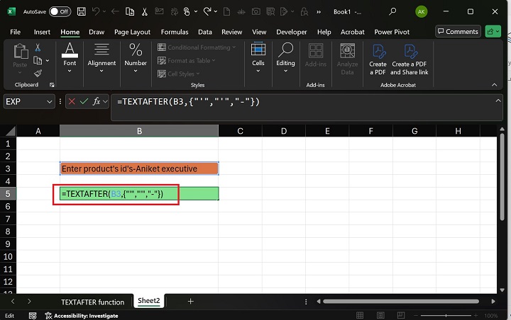
Therefore, the TEXTAFTER function will extract the text after the first delimiter in the given string.
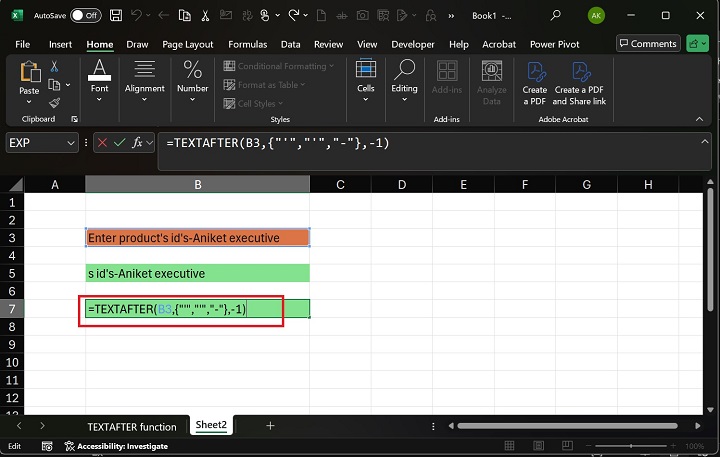
In another scenario, if you wish to obtain the text after the last delimiter, you can set the instance_num to -1. Write the formula =TEXTAFTER(B3,{"'","'","-"},-1) in the B7cell and hit the Enter button.
Example 3
If the delimiter is not matched in the text string, use the TEXTAFTER function to write your message.
Solution
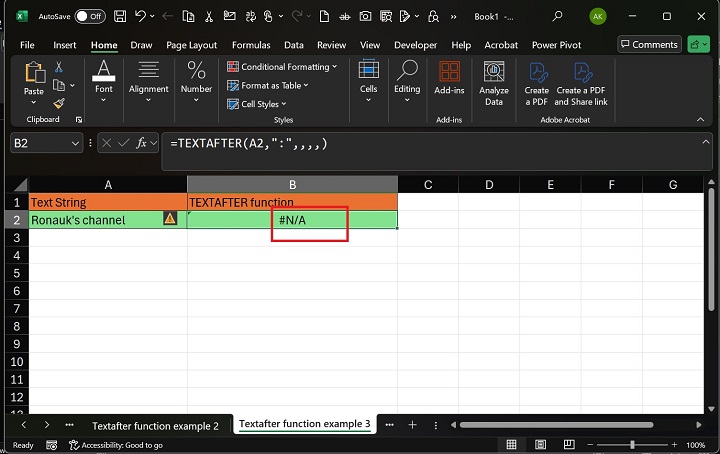
The TEXTAFTER function retrieves the #N/A error if the delimiter is unavailable in the text string. In the below screenshot, the colon : delimiter is not present in the A2 cell.
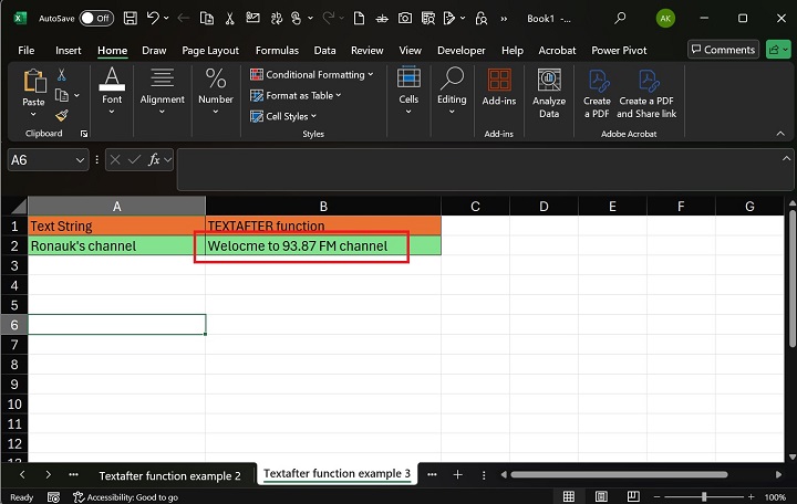
Now, modify the formula =TEXTAFTER(A2,":",,,,"Welcome to 93.68 channel") in the B2 cell and hit the Enter.
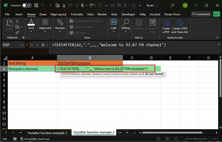
Therefore, the TEXTAFTER function will retrieve the message Welcome to 93.87 FM channel you wrote in the sixth argument.
Example 4
Set the match_mode to 1 for case insensitivity.
Solution
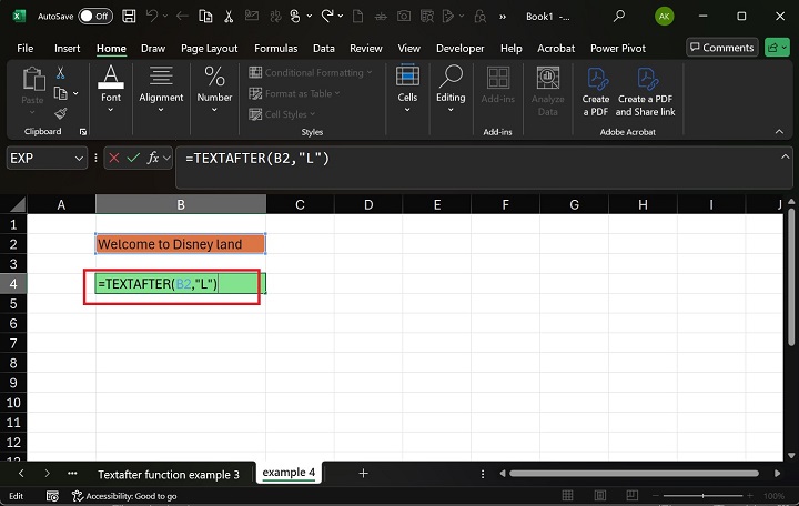
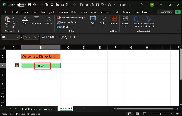
The TEXTAFTER function distinguishes uppercase and lowercase differently. Suppose you provide text in lowercase in the second argument, but the text is uppercase in the input string. This function retrieves the #N/A error because the exact match is not identified in the TEXTAFTER function. Write the formula =TEXTAFTER(B2,"L") in the B4 cell.
Once you hit Enter, the TEXTAFTER function will return the #N/A error.
To ignore the case insensitivity, you can set the match_mode to 1. Write the formula =TEXTAFTER(B2,"L",,1) in the B4 cell and press the Enter tab.
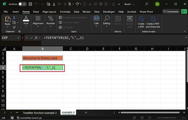
Therefore, the TEXTAFTER function will retrieve the text come to Disney land, where the case insensitivity has been ignored.

Download Practice Sheet
You can download and use the sample data sheet to practice the TEXTAFTER function.
