- Digital Image Processing
- DIP - Home
- DIP - Image Processing Introduction
- DIP - Signal and System Introduction
- DIP - History of Photography
- DIP - Applications and Usage
- DIP - Concept of Dimensions
- DIP - Image Formation on Camera
- DIP - Camera Mechanism
- DIP - Concept of Pixel
- DIP - Perspective Transformation
- DIP - Concept of Bits Per Pixel
- DIP - Types of Images
- DIP - Color Codes Conversion
- DIP - Grayscale to RGB Conversion
- DIP - Concept of Sampling
- DIP - Pixel Resolution
- DIP - Concept of Zooming
- DIP - Zooming methods
- DIP - Spatial Resolution
- DIP - Pixels Dots and Lines per inch
- DIP - Gray Level Resolution
- DIP - Concept of Quantization
- DIP - ISO Preference curves
- DIP - Concept of Dithering
- DIP - Histograms Introduction
- DIP - Brightness and Contrast
- DIP - Image Transformations
- DIP - Histogram Sliding
- DIP - Histogram Stretching
- DIP - Introduction to Probability
- DIP - Histogram Equalization
- DIP - Gray Level Transformations
- DIP - Concept of convolution
- DIP - Concept of Masks
- DIP - Concept of Blurring
- DIP - Concept of Edge Detection
- DIP - Prewitt Operator
- DIP - Sobel operator
- DIP - Robinson Compass Mask
- DIP - Krisch Compass Mask
- DIP - Laplacian Operator
- DIP - Frequency Domain Analysis
- DIP - Fourier series and Transform
- DIP - Convolution theorm
- DIP - High Pass vs Low Pass Filters
- DIP - Introduction to Color Spaces
- DIP - JPEG compression
- DIP - Optical Character Recognition
- DIP - Computer Vision and Graphics
- DIP Useful Resources
- DIP - Quick Guide
- DIP - Useful Resources
- DIP - Discussion
DIP - Quick Guide
Digital Image Processing Introduction
Introduction
Signal processing is a discipline in electrical engineering and in mathematics that deals with analysis and processing of analog and digital signals , and deals with storing , filtering , and other operations on signals. These signals include transmission signals , sound or voice signals , image signals , and other signals e.t.c.
Out of all these signals , the field that deals with the type of signals for which the input is an image and the output is also an image is done in image processing. As it name suggests, it deals with the processing on images.
It can be further divided into analog image processing and digital image processing.
Analog image processing
Analog image processing is done on analog signals. It includes processing on two dimensional analog signals. In this type of processing, the images are manipulated by electrical means by varying the electrical signal. The common example include is the television image.
Digital image processing has dominated over analog image processing with the passage of time due its wider range of applications.
Digital image processing
The digital image processing deals with developing a digital system that performs operations on an digital image.
What is an Image
An image is nothing more than a two dimensional signal. It is defined by the mathematical function f(x,y) where x and y are the two co-ordinates horizontally and vertically.
The value of f(x,y) at any point is gives the pixel value at that point of an image.
The above figure is an example of digital image that you are now viewing on your computer screen. But actually , this image is nothing but a two dimensional array of numbers ranging between 0 and 255.
| 128 | 30 | 123 |
| 232 | 123 | 321 |
| 123 | 77 | 89 |
| 80 | 255 | 255 |
Each number represents the value of the function f(x,y) at any point. In this case the value 128 , 230 ,123 each represents an individual pixel value. The dimensions of the picture is actually the dimensions of this two dimensional array.
Relationship between a digital image and a signal
If the image is a two dimensional array then what does it have to do with a signal? In order to understand that , We need to first understand what is a signal?
Signal
In physical world, any quantity measurable through time over space or any higher dimension can be taken as a signal. A signal is a mathematical function, and it conveys some information. A signal can be one dimensional or two dimensional or higher dimensional signal. One dimensional signal is a signal that is measured over time. The common example is a voice signal. The two dimensional signals are those that are measured over some other physical quantities. The example of two dimensional signal is a digital image. We will look in more detail in the next tutorial of how a one dimensional or two dimensional signals and higher signals are formed and interpreted.
Relationship
Since anything that conveys information or broadcast a message in physical world between two observers is a signal. That includes speech or (human voice) or an image as a signal. Since when we speak , our voice is converted to a sound wave/signal and transformed with respect to the time to person we are speaking to. Not only this , but the way a digital camera works, as while acquiring an image from a digital camera involves transfer of a signal from one part of the system to the other.
How a digital image is formed
Since capturing an image from a camera is a physical process. The sunlight is used as a source of energy. A sensor array is used for the acquisition of the image. So when the sunlight falls upon the object, then the amount of light reflected by that object is sensed by the sensors, and a continuous voltage signal is generated by the amount of sensed data. In order to create a digital image , we need to convert this data into a digital form. This involves sampling and quantization. (They are discussed later on). The result of sampling and quantization results in an two dimensional array or matrix of numbers which are nothing but a digital image.
Overlapping fields
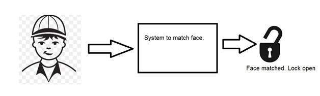
Machine/Computer vision
Machine vision or computer vision deals with developing a system in which the input is an image and the output is some information. For example: Developing a system that scans human face and opens any kind of lock. This system would look something like this.
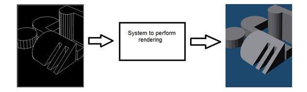
Computer graphics
Computer graphics deals with the formation of images from object models, rather then the image is captured by some device. For example: Object rendering. Generating an image from an object model. Such a system would look something like this.
Artificial intelligence
Artificial intelligence is more or less the study of putting human intelligence into machines. Artificial intelligence has many applications in image processing. For example: developing computer aided diagnosis systems that help doctors in interpreting images of X-ray , MRI e.t.c and then highlighting conspicuous section to be examined by the doctor.
Signal processing
Signal processing is an umbrella and image processing lies under it. The amount of light reflected by an object in the physical world (3d world) is pass through the lens of the camera and it becomes a 2d signal and hence result in image formation. This image is then digitized using methods of signal processing and then this digital image is manipulated in digital image processing.
Signals and Systems Introduction
This tutorial covers the basics of signals and system necessary for understanding the concepts of digital image processing. Before going into the detail concepts , lets first define the simple terms.
Signals
In electrical engineering, the fundamental quantity of representing some information is called a signal. It doesnot matter what the information is i-e: Analog or digital information. In mathematics, a signal is a function that conveys some information. In fact any quantity measurable through time over space or any higher dimension can be taken as a signal. A signal could be of any dimension and could be of any form.
Analog signals
A signal could be an analog quantity that means it is defined with respect to the time. It is a continuous signal. These signals are defined over continuous independent variables. They are difficult to analyze, as they carry a huge number of values. They are very much accurate due to a large sample of values. In order to store these signals , you require an infinite memory because it can achieve infinite values on a real line. Analog signals are denoted by sin waves.
For example:
Human voice
Human voice is an example of analog signals. When you speak , the voice that is produced travel through air in the form of pressure waves and thus belongs to a mathematical function, having independent variables of space and time and a value corresponding to air pressure.
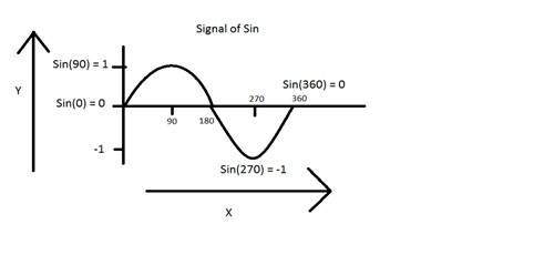
Another example is of sin wave which is shown in the figure below.
Y = sin(x) where x is indepedent
Digital signals
As compared to analog signals, digital signals are very easy to analyze. They are discontinuous signals. They are the appropriation of analog signals.
The word digital stands for discrete values and hence it means that they use specific values to represent any information. In digital signal , only two values are used to represent something i-e: 1 and 0 (binary values). Digital signals are less accurate then analog signals because they are the discrete samples of an analog signal taken over some period of time. However digital signals are not subject to noise. So they last long and are easy to interpret. Digital signals are denoted by square waves.
For example:
Computer keyboard
Whenever a key is pressed from the keyboard , the appropriate electrical signal is sent to keyboard controller containing the ASCII value that particular key. For example the electrical signal that is generated when keyboard key a is pressed, carry information of digit 97 in the form of 0 and 1, which is the ASCII value of character a.
Difference between analog and digital signals
| Comparison element | Analog signal | Digital signal |
|---|---|---|
| Analysis | Difficult | Possible to analyze |
| Representation | Continuous | Discontinuous |
| Accuracy | More accurate | Less accurate |
| Storage | Infinite memory | Easily stored |
| Subject to Noise | Yes | No |
| Recording Technique | Original signal is preserved | Samples of the signal are taken and preserved |
| Examples | Human voice , Thermometer , Analog phones e.t.c | Computers , Digital Phones , Digital pens , e.t.c |
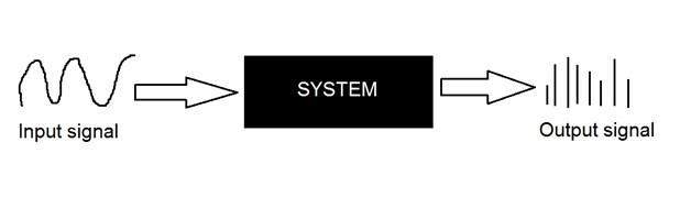
Systems
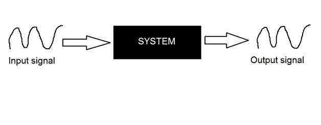
A system is a defined by the type of input and output it deals with. Since we are dealing with signals , so in our case , our system would be a mathematical model , a piece of code/software , or a physical device , or a black box whose input is a signal and it performs some processing on that signal , and the output is a signal. The input is known as excitation and the output is known as response.

In the above figure a system has been shown whose input and output both are signals but the input is an analog signal. And the output is an digital signal. It means our system is actually a conversion system that converts analog signals to digital signals.
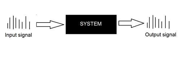
Lets have a look at the inside of this black box system
Conversion of analog to digital signals
Since there are lot of concepts related to this analog to digital conversion and vice-versa. We will only discuss those which are related to digital image processing. There are two main concepts that are involved in the coversion.
Sampling
Quantization
Sampling
Sampling as its name suggests can be defined as take samples. Take samples of a digital signal over x axis. Sampling is done on an independent variable. In case of this mathematical equation:
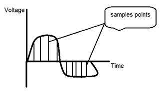
Sampling is done on the x variable. We can also say that the conversion of x axis (infinite values) to digital is done under sampling.
Sampling is further divide into up sampling and down sampling. If the range of values on x-axis are less then we will increase the sample of values. This is known as up sampling and its vice versa is known as down sampling
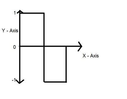
Quantization
Quantization as its name suggest can be defined as dividing into quanta (partitions). Quantization is done on dependent variable. It is opposite to sampling.
In case of this mathematical equation y = sin(x)
Quantization is done on the Y variable. It is done on the y axis. The conversion of y axis infinite values to 1 , 0 , -1 (or any other level) is known as Quantization.
These are the two basics steps that are involved while converting an analog signal to a digital signal.
The quantization of a signal has been shown in the figure below.
Why do we need to convert an analog signal to digital signal.
The first and obvious reason is that digital image processing deals with digital images , that are digital signals. So when ever the image is captured , it is converted into digital format and then it is processed.
The second and important reason is , that in order to perform operations on an analog signal with a digital computer , you have to store that analog signal in the computer. And in order to store an analog signal , infinite memory is required to store it. And since thats not possible , so thats why we convert that signal into digital format and then store it in digital computer and then performs operations on it.
Continuous systems vs discrete systems
Continuous systems
The type of systems whose input and output both are continuous signals or analog signals are called continuous systems.
Discrete systems
The type of systems whose input and output both are discrete signals or digital signals are called digital systems
History of Photography
Origin of camera
The history of camera and photography is not exactly the same. The concepts of camera were introduced a lot before the concept of photography
Camera Obscura
The history of the camera lies in ASIA. The principles of the camera were first introduced by a Chinese philosopher MOZI. It is known as camera obscura. The cameras evolved from this principle.
The word camera obscura is evolved from two different words. Camera and Obscura. The meaning of the word camera is a room or some kind of vault and Obscura stands for dark.
The concept which was introduced by the Chinese philosopher consist of a device, that project an image of its surrounding on the wall. However it was not built by the Chinese.
The creation of camera obscura
The concept of Chinese was bring in reality by a Muslim scientist Abu Ali Al-Hassan Ibn al-Haitham commonly known as Ibn al-Haitham. He built the first camera obscura. His camera follows the principles of pinhole camera. He build this device in somewhere around 1000.
Portable camera
In 1685, a first portable camera was built by Johann Zahn. Before the advent of this device , the camera consist of a size of room and were not portable. Although a device was made by an Irish scientist Robert Boyle and Robert Hooke that was a transportable camera, but still that device was very huge to carry it from one place to the other.
Origin of photography
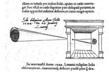
Although the camera obscura was built in 1000 by a Muslim scientist. But its first actual use was described in the 13th century by an English philosopher Roger Bacon. Roger suggested the use of camera for the observation of solar eclipses.
Da Vinci
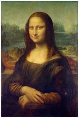
Although much improvement has been made before the 15th century , but the improvements and the findings done by Leonardo di ser Piero da Vinci was remarkable. Da Vinci was a great artist , musician , anatomist , and a war enginner. He is credited for many inventions. His one of the most famous painting includes, the painting of Mona Lisa.
Da vinci not only built a camera obscura following the principle of a pin hole camera but also uses it as drawing aid for his art work. In his work , which was described in Codex Atlanticus , many principles of camera obscura has been defined.
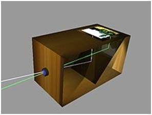
His camera follows the principle of a pin hole camera which can be described as
When images of illuminated objects penetrate through a small hole into a very dark room you will see [on the opposite wall] these objects in their proper form and color, reduced in size in a reversed position, owing to the intersection of rays.
First photograph
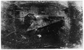
The first photograph was taken in 1814 by a French inventor Joseph Nicephore Niepce. He captures the first photograph of a view from the window at Le Gras, by coating the pewter plate with bitumen and after that exposing that plate to light.
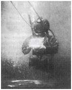
First underwater photograph
The first underwater photograph was taken by an English mathematician William Thomson using a water tight box. This was done in 1856.
The origin of film
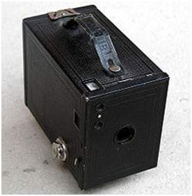
The origin of film was introduced by an American inventor and a philanthropist known as George Eastman who is considered as the pioneer of photography.
He founded the company called as Eastman Kodak , which is famous for developing films. The company starts manufacturing paper film in 1885. He first created the camera Kodak and then later Brownie. Brownie was a box camera and gain its popularity due to its feature of Snapshot.
After the advent of the film , the camera industry once again got a boom and one invention lead to another.
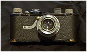
Leica and Argus
Leica and argus are the two analog cameras developed in 1925 and in 1939 respectively. The camera Leica was built using a 35mm cine film.
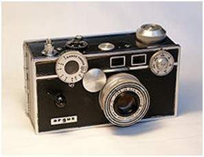
Argus was another camera analog camera that uses the 35mm format and was rather inexpensive as compared by Leica and became very popular.
Analog CCTV cameras
In 1942 a German engineer Walter Bruch developed and installed the very first system of the analog CCTV cameras. He is also credited for the invention of color television in the 1960.
Photo Pac
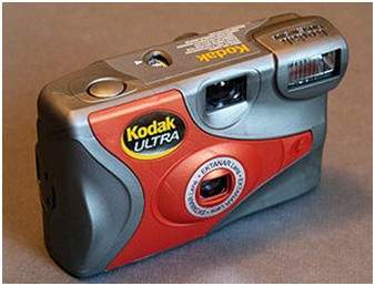
The first disposable camera was introduced in 1949 by Photo Pac. The camera was only a one time use camera with a roll of film already included in it. The later versions of Photo pac were water proof and even have the flash.
Digital Cameras
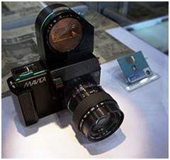
Mavica by Sony
Mavica (the magnetic video camera) was launched by Sony in 1981 was the first game changer in digital camera world. The images were recorded on floppy disks and images can be viewed later on any monitor screen.
It was not a pure digital camera , but an analog camera. But got its popularity due to its storing capacity of images on a floppy disks. It means that you can now store images for a long lasting period , and you can save a huge number of pictures on the floppy which are replaced by the new blank disc , when they got full. Mavica has the capacity of storing 25 images on a disk.
One more important thing that mavica introduced was its 0.3 mega pixel capacity of capturing photos.
Digital Cameras
Fuji DS-1P camera by Fuji films 1988 was the first true digital camera
Nikon D1 was a 2.74 mega pixel camera and the first commercial digital SLR camera developed by Nikon , and was very much affordable by the professionals.
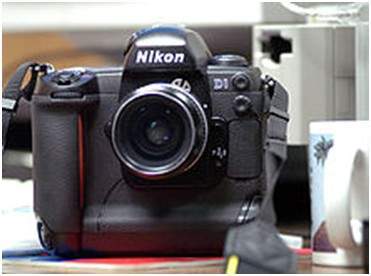
Today digital cameras are included in the mobile phones with very high resolution and quality.
Applications and Usage
Since digital image processing has very wide applications and almost all of the technical fields are impacted by DIP, we will just discuss some of the major applications of DIP.
Digital Image processing is not just limited to adjust the spatial resolution of the everyday images captured by the camera. It is not just limited to increase the brightness of the photo, e.t.c. Rather it is far more than that.
Electromagnetic waves can be thought of as stream of particles, where each particle is moving with the speed of light. Each particle contains a bundle of energy. This bundle of energy is called a photon.
The electromagnetic spectrum according to the energy of photon is shown below.
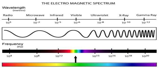
In this electromagnetic spectrum, we are only able to see the visible spectrum. Visible spectrum mainly includes seven different colors that are commonly term as (VIBGOYR). VIBGOYR stands for violet , indigo , blue , green , orange , yellow and Red.
But that doesnot nullify the existence of other stuff in the spectrum. Our human eye can only see the visible portion, in which we saw all the objects. But a camera can see the other things that a naked eye is unable to see. For example: x rays , gamma rays , e.t.c. Hence the analysis of all that stuff too is done in digital image processing.
This discussion leads to another question which is
why do we need to analyze all that other stuff in EM spectrum too?
The answer to this question lies in the fact, because that other stuff such as XRay has been widely used in the field of medical. The analysis of Gamma ray is necessary because it is used widely in nuclear medicine and astronomical observation. Same goes with the rest of the things in EM spectrum.
Applications of Digital Image Processing
Some of the major fields in which digital image processing is widely used are mentioned below
Image sharpening and restoration
Medical field
Remote sensing
Transmission and encoding
Machine/Robot vision
Color processing
Pattern recognition
Video processing
Microscopic Imaging
Others
Image sharpening and restoration
Image sharpening and restoration refers here to process images that have been captured from the modern camera to make them a better image or to manipulate those images in way to achieve desired result. It refers to do what Photoshop usually does.
This includes Zooming, blurring , sharpening , gray scale to color conversion, detecting edges and vice versa , Image retrieval and Image recognition. The common examples are:
The original image

The zoomed image
Blurr image
Sharp image
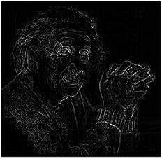
Edges
Medical field
The common applications of DIP in the field of medical is
Gamma ray imaging
PET scan
X Ray Imaging
Medical CT
UV imaging
UV imaging
In the field of remote sensing , the area of the earth is scanned by a satellite or from a very high ground and then it is analyzed to obtain information about it. One particular application of digital image processing in the field of remote sensing is to detect infrastructure damages caused by an earthquake.
As it takes longer time to grasp damage, even if serious damages are focused on. Since the area effected by the earthquake is sometimes so wide , that it not possible to examine it with human eye in order to estimate damages. Even if it is , then it is very hectic and time consuming procedure. So a solution to this is found in digital image processing. An image of the effected area is captured from the above ground and then it is analyzed to detect the various types of damage done by the earthquake.
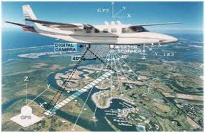
The key steps include in the analysis are
The extraction of edges
Analysis and enhancement of various types of edges
Transmission and encoding
The very first image that has been transmitted over the wire was from London to New York via a submarine cable. The picture that was sent is shown below.
The picture that was sent took three hours to reach from one place to another.
Now just imagine , that today we are able to see live video feed , or live cctv footage from one continent to another with just a delay of seconds. It means that a lot of work has been done in this field too. This field doesnot only focus on transmission , but also on encoding. Many different formats have been developed for high or low bandwith to encode photos and then stream it over the internet or e.t.c.
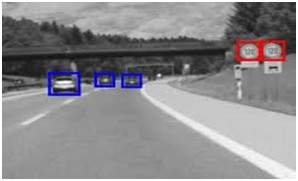
Machine/Robot vision
Apart form the many challenges that a robot face today , one of the biggest challenge still is to increase the vision of the robot. Make robot able to see things , identify them , identify the hurdles e.t.c. Much work has been contributed by this field and a complete other field of computer vision has been introduced to work on it.
Hurdle detection
Hurdle detection is one of the common task that has been done through image processing, by identifying different type of objects in the image and then calculating the distance between robot and hurdles.
Line follower robot
Most of the robots today work by following the line and thus are called line follower robots. This help a robot to move on its path and perform some tasks. This has also been achieved through image processing.
Color processing
Color processing includes processing of colored images and different color spaces that are used. For example RGB color model , YCbCr, HSV. It also involves studying transmission , storage , and encoding of these color images.
Pattern recognition
Pattern recognition involves study from image processing and from various other fields that includes machine learning ( a branch of artificial intelligence). In pattern recognition , image processing is used for identifying the objects in an images and then machine learning is used to train the system for the change in pattern. Pattern recognition is used in computer aided diagnosis , recognition of handwriting , recognition of images e.t.c
Video processing
A video is nothing but just the very fast movement of pictures. The quality of the video depends on the number of frames/pictures per minute and the quality of each frame being used. Video processing involves noise reduction , detail enhancement , motion detection , frame rate conversion , aspect ratio conversion , color space conversion e.t.c.
Concept of Dimensions
We will look at this example in order to understand the concept of dimension.
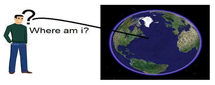
Consider you have a friend who lives on moon, and he wants to send you a gift on your birthday present. He ask you about your residence on earth. The only problem is that the courier service on moon doesnot understand the alphabetical address, rather it only understand the numerical co-ordinates. So how do you send him your position on earth?
Thats where comes the concept of dimensions. Dimensions define the minimum number of points required to point a position of any particular object within a space.
So lets go back to our example again in which you have to send your position on earth to your friend on moon. You send him three pair of co-ordinates. The first one is called longitude , the second one is called latitude, and the third one is called altitude.
These three co-ordinates define your position on the earth. The first two defines your location , and the third one defines your height above the sea level.
So that means that only three co-ordinates are required to define your position on earth. That means you live in world which is 3 dimensional. And thus this not only answers the question about dimension , but also answers the reason , that why we live in a 3d world.
Since we are studying this concept in reference to the digital image processing, so we are now going to relate this concept of dimension with an image.
Dimensions of image
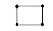
So if we live in the 3d world , means a 3 dimensional world, then what are the dimensions of an image that we capture. An image is a two dimensional, thats why we also define an image as a 2 dimensional signal. An image has only height and width. An image doesnot have depth. Just have a look at this image below.
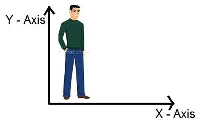
If you would look at the above figure , it shows that it has only two axis which are the height and width axis. You cannot perceive depth from this image. Thats why we say that an image is two dimensional signal. But our eye is able to perceive three dimensional objects , but this would be more explained in the next tutorial of how the camera works , and image is perceived.
This discussion leads to some other questions that how 3 dimension systems is formed from 2 dimension.
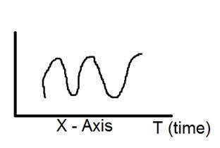
How does television works?
If we look the image above , we will see that it is a two dimensional image. In order to convert it into three dimension , we need one other dimension. Lets take time as the third dimension , in that case we will move this two dimensional image over the third dimension time. The same concept that happens in television, that helps us perceive the depth of different objects on a screen. Does that mean that what comes on the T.V or what we see in the television screen is 3d. Well we can yes. The reason is that, in case of T.V we if we are playing a video. Then a video is nothing else but two dimensional pictures move over time dimension. As two dimensional objects are moving over the third dimension which is a time so we can say it is 3 dimensional.
Different dimensions of signals
1 dimension signal
The common example of a 1 dimension signal is a waveform. It can be mathematically represented as
F(x) = waveform
Where x is an independent variable. Since it is a one dimension signal , so thats why there is only one variable x is used.
Pictorial representation of a one dimensional signal is given below:
The above figure shows a one dimensional signal.
Now this lead to another question, which is, even though it is a one dimensional signal ,then why does it have two axis?. The answer to this question is that even though it is a one dimensional signal , but we are drawing it in a two dimensional space. Or we can say that the space in which we are representing this signal is two dimensional. Thats why it looks like a two dimensional signal.
Perhaps you can understand the concept of one dimension more better by looking at the figure below.
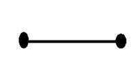
Now refer back to our initial discussion on dimension, Consider the above figure a real line with positive numbers from one point to the other. Now if we have to explain the location of any point on this line, we just need only one number, which means only one dimension.
2 dimensions signal
The common example of a two dimensional signal is an image , which has already been discussed above.

As we have already seen that an image is two dimensional signal, i-e: it has two dimensions. It can be mathematically represented as:
F (x , y) = Image
Where x and y are two variables. The concept of two dimension can also be explained in terms of mathematics as:
Now in the above figure, label the four corners of the square as A,B,C and D respectively. If we call , one line segment in the figure AB and the other CD , then we can see that these two parallel segments join up and make a square. Each line segment corresponds to one dimension , so these two line segments correspond to 2 dimensions.
3 dimension signal
Three dimensional signal as it names refers to those signals which has three dimensions. The most common example has been discussed in the beginning which is of our world. We live in a three dimensional world. This example has been discussed very elaborately. Another example of a three dimensional signal is a cube or a volumetric data or the most common example would be animated or 3d cartoon character.
The mathematical representation of three dimensional signal is:
F(x,y,z) = animated character.
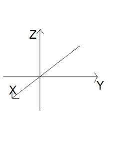
Another axis or dimension Z is involved in a three dimension, that gives the illusion of depth. In a Cartesian co-ordinate system it can be viewed as:
4 dimension signal
In a four dimensional signal , four dimensions are involved. The first three are the same as of three dimensional signal which are: (X, Y, Z), and the fourth one which is added to them is T(time). Time is often referred to as temporal dimension which is a way to measure change. Mathematically a four d signal can be stated as:
F(x,y,z,t) = animated movie.
The common example of a 4 dimensional signal can be an animated 3d movie. As each character is a 3d character and then they are moved with respect to the time, due to which we saw an illusion of a three dimensional movie more like a real world.
So that means that in reality the animated movies are 4 dimensional i-e: movement of 3d characters over the fourth dimension time.
Image Formation on Camera
How human eye works?
Before we discuss , the image formation on analog and digital cameras , we have to first discuss the image formation on human eye. Because the basic principle that is followed by the cameras has been taken from the way , the human eye works.
When light falls upon the particular object , it is reflected back after striking through the object. The rays of light when passed through the lens of eye , form a particular angle , and the image is formed on the retina which is the back side of the wall. The image that is formed is inverted. This image is then interpreted by the brain and that makes us able to understand things. Due to angle formation , we are able to perceive the height and depth of the object we are seeing. This has been more explained in the tutorial of perspective transformation.
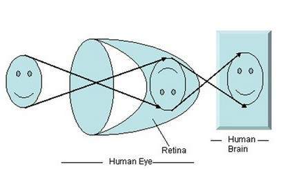
As you can see in the above figure, that when sun light falls on the object (in this case the object is a face), it is reflected back and different rays form different angle when they are passed through the lens and an invert image of the object has been formed on the back wall. The last portion of the figure denotes that the object has been interpreted by the brain and re-inverted.
Now lets take our discussion back to the image formation on analog and digital cameras.
Image formation on analog cameras
In analog cameras , the image formation is due to the chemical reaction that takes place on the strip that is used for image formation.
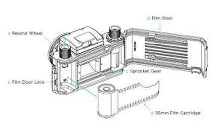
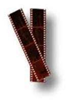
A 35mm strip is used in analog camera. It is denoted in the figure by 35mm film cartridge. This strip is coated with silver halide ( a chemical substance).
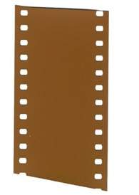
A 35mm strip is used in analog camera. It is denoted in the figure by 35mm film cartridge. This strip is coated with silver halide ( a chemical substance).
Light is nothing but just the small particles known as photon particles.So when these photon particles are passed through the camera, it reacts with the silver halide particles on the strip and it results in the silver which is the negative of the image.
In order to understand it better , have a look at this equation.
Photons (light particles) + silver halide ? silver ? image negative.
This is just the basics, although image formation involves many other concepts regarding the passing of light inside , and the concepts of shutter and shutter speed and aperture and its opening but for now we will move on to the next part. Although most of these concepts have been discussed in our tutorial of shutter and aperture.
This is just the basics, although image formation involves many other concepts regarding the passing of light inside , and the concepts of shutter and shutter speed and aperture and its opening but for now we will move on to the next part. Although most of these concepts have been discussed in our tutorial of shutter and aperture.
Image formation on digital cameras
In the digital cameras , the image formation is not due to the chemical reaction that take place , rather it is a bit more complex then this. In the digital camera , a CCD array of sensors is used for the image formation.
Image formation through CCD array
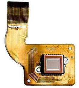
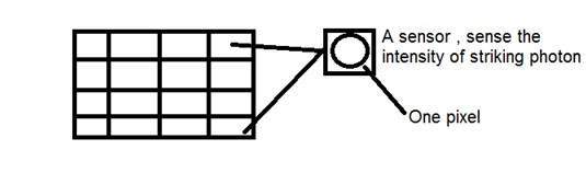
CCD stands for charge-coupled device. It is an image sensor, and like other sensors it senses the values and converts them into an electric signal. In case of CCD it senses the image and convert it into electric signal e.t.c.
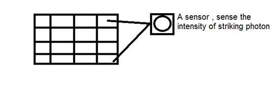
This CCD is actually in the shape of array or a rectangular grid. It is like a matrix with each cell in the matrix contains a censor that senses the intensity of photon.
Like analog cameras , in the case of digital too , when light falls on the object , the light reflects back after striking the object and allowed to enter inside the camera.
Each sensor of the CCD array itself is an analog sensor. When photons of light strike on the chip , it is held as a small electrical charge in each photo sensor. The response of each sensor is directly equal to the amount of light or (photon) energy striked on the surface of the sensor.
Since we have already define an image as a two dimensional signal and due to the two dimensional formation of the CCD array , a complete image can be achieved from this CCD array.
It has limited number of sensors , and it means a limited detail can be captured by it. Also each sensor can have only one value against the each photon particle that strike on it.
So the number of photons striking(current) are counted and stored. In order to measure accurately these , external CMOS sensors are also attached with CCD array.
Introduction to pixel
The value of each sensor of the CCD array refers to each the value of the individual pixel. The number of sensors = number of pixels. It also means that each sensor could have only one and only one value.
Storing image
The charges stored by the CCD array are converted to voltage one pixel at a time. With the help of additional circuits , this voltage is converted into a digital information and then it is stored.
Each company that manufactures digital camera, make their own CCD sensors. That include , Sony , Mistubishi , Nikon ,Samsung , Toshiba , FujiFilm , Canon e.t.c.
Apart from the other factors , the quality of the image captured also depends on the type and quality of the CCD array that has been used.
Camera Mechansim
In this tutorial, we will discuss some of the basic camera concepts, like aperture , shutter , shutter speed , ISO and we will discuss the collective use of these concepts to capture a good image.
Aperture
Aperture is a small opening which allows the light to travel inside into camera. Here is the picture of aperture.
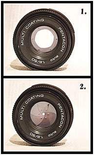
You will see some small blades like stuff inside the aperture. These blades create a octagonal shape that can be opened closed. And thus it make sense that , the more blades will open, the hole from which the light would have to pass would be bigger. The bigger the hole , the more light is allowed to enter.
Effect
The effect of the aperture directly corresponds to brightness and darkness of an image. If the aperture opening is wide , it would allow more light to pass into the camera. More light would result in more photons, which ultimately result in a brighter image.
The example of this is shown below
Consider these two photos
The one on the right side looks brighter, it means that when it was captured by the camera , the aperture was wide open. As compare to the other picture on the left side , which is very dark as compare to the first one, that shows that when that image was captured, its aperture was not wide open.
Size
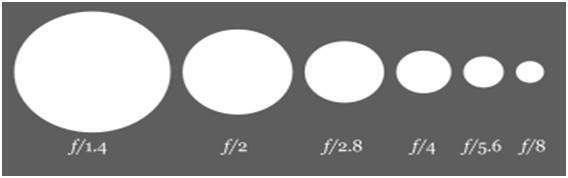
Now lets discuss the maths behind the aperture. The size of the aperture is denoted by a f value. And it is inversely proportional to the opening of aperture.
Here are the two equations , that best explain this concept.
Large aperture size = Small f value
Small aperture size = Greater f value
Pictorially it can be represented as:
Shutter
After the aperture , there comes the shutter. The light when allowed to pass from the aperture , falls directly on to the shutter. Shutter is actually a cover, a closed window , or can be thought of as a curtain. Remember when we talk about the CCD array sensor on which the image is formed. Well behind the shutter is the sensor. So shutter is the only thing that is between the image formation and the light , when it is passed from aperture.
As soon as the shutter is open , light falls on the image sensor , and the image is formed on the array.
Effect
If the shutter allows light to pass a bit longer , the image would be brighter. Similarly a darker picture is produced , when a shutter is allowed to move very quickly and hence, the light that is allowed to pass has very less photons , and the image that is formed on the CCD array sensor is very dark.
Shutter has further two main concepts:
Shutter Speed
Shutter time
Shutter speed
The shutter speed can be referred to as the number of times the shutter get open or close. Remember we are not talking about for how long the shutter get open or close.
Shutter time
The shutter time can be defined as
When the shutter is open , then the amount of wait time it take till it is closed is called shutter time.
In this case we are not talking about how many times , the shutter got open or close , but we are talking about for how much time does it remain wide open.
For example:
We can better understand these two concepts in this way. That lets say that a shutter opens 15 times and then get closed, and for each time it opens for 1 second and then get closed. In this example , 15 is the shutter speed and 1 second is the shutter time.
Relationship
The relationship between shutter speed and shutter time is that they are both inversely proportional to each other.
This relationship can be defined in the equation below.
More shutter speed = less shutter time
Less shutter speed = more shutter time.
Explanation:
The lesser the time required , the more is the speed. And the greater the time required , the less is the speed.
Applications
These two concepts together make a variety of applications. Some of them are given below.
Fast moving objects:
If you were to capture the image of a fast moving object , could be a car or anything. The adjustment of shutter speed and its time would effect a lot.
So , in order to capture an image like this, we will make two amendments:
Increase shutter speed
Decrease shutter time
What happens is , that when we increase shutter speed , the more number of times , the shutter would open or close. It means different samples of light would allow to pass in. And when we decrease shutter time , it means we will immediately captures the scene, and close the shutter gate.
If you will do this , you get a crisp image of a fast moving object.
In order to understand it , we will look at this example. Suppose you want to capture the image of fast moving water fall.
You set your shutter speed to 1 second and you capture a photo. This is what you get
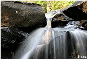
Then you set your shutter speed to a faster speed and you get.
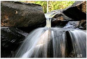
Then again you set your shutter speed to even more faster and you get.
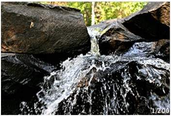
You can see in the last picture , that we have increase our shutter speed to very fast, that means that a shutter get opened or closed in 200th of 1 second and so we got a crisp image.
ISO
ISO factor is measured in numbers. It denotes the sensitivity of light to camera. If ISO number is lowered , it means our camera is less sensitive to light and if the ISO number is high, it means it is more senstivie.
Effect
The higher is the ISO , the more brighter the picture would be. IF ISO is set to 1600 , the picture would be very brighter and vice versa.
Side effect
If the ISO increases, the noise in the image also increases. Today most of the camera manufacturing companies are working on removing the noise from the image when ISO is set to higher speed.
Concept of Pixel
Pixel
Pixel is the smallest element of an image. Each pixel correspond to any one value. In an 8-bit gray scale image, the value of the pixel between 0 and 255. The value of a pixel at any point correspond to the intensity of the light photons striking at that point. Each pixel store a value proportional to the light intensity at that particular location.
PEL
A pixel is also known as PEL. You can have more understanding of the pixel from the pictures given below.
In the above picture, there may be thousands of pixels, that together make up this image. We will zoom that image to the extent that we are able to see some pixels division. It is shown in the image below.

In the above picture, there may be thousands of pixels, that together make up this image. We will zoom that image to the extent that we are able to see some pixels division. It is shown in the image below.
Relation ship with CCD array
We have seen that how an image is formed in the CCD array. So a pixel can also be defined as
The smallest division the CCD array is also known as pixel.
Each division of CCD array contains the value against the intensity of the photon striking to it. This value can also be called as a pixel
Calculation of total number of pixels
We have define an image as a two dimensional signal or matrix. Then in that case the number of PEL would be equal to the number of rows multiply with number of columns.
This can be mathematically represented as below:
Total number of pixels = number of rows ( X ) number of columns
Or we can say that the number of (x,y) coordinate pairs make up the total number of pixels.
We will look in more detail in the tutorial of image types , that how do we calculate the pixels in a color image.
Gray level
The value of the pixel at any point denotes the intensity of image at that location , and that is also known as gray level.
We will see in more detail about the value of the pixels in the image storage and bits per pixel tutorial, but for now we will just look at the concept of only one pixel value.
Pixel value.(0)
As it has already been define in the beginning of this tutorial , that each pixel can have only one value and each value denotes the intensity of light at that point of the image.
We will now look at a very unique value 0. The value 0 means absence of light. It means that 0 denotes dark, and it further means that when ever a pixel has a value of 0, it means at that point , black color would be formed.
Have a look at this image matrix
| 0 | 0 | 0 |
| 0 | 0 | 0 |
| 0 | 0 | 0 |
Now this image matrix has all filled up with 0. All the pixels have a value of 0. If we were to calculate the total number of pixels form this matrix , this is how we are going to do it.
Total no of pixels = total no. of rows X total no. of columns
= 3 X 3
= 9.
It means that an image would be formed with 9 pixels, and that image would have a dimension of 3 rows and 3 column and most importantly that image would be black.
The resulting image that would be made would be something like this

Now why is this image all black. Because all the pixels in the image had a value of 0.
Perspective Transformation
When human eyes see near things they look bigger as compare to those who are far away. This is called perspective in a general way. Whereas transformation is the transfer of an object e.t.c from one state to another.
So overall , the perspective transformation deals with the conversion of 3d world into 2d image. The same principle on which human vision works and the same principle on which the camera works.
We will see in detail about why this happens , that those objects which are near to you look bigger , while those who are far away , look smaller even though they look bigger when you reach them.
We will start this discussion by the concept of frame of reference:
Frame of reference:
Frame of reference is basically a set of values in relation to which we measure something.
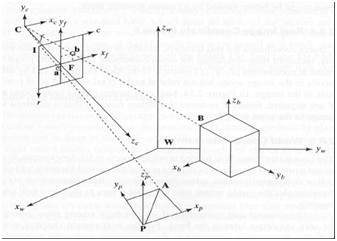
5 frames of reference
In order to analyze a 3d world/image/scene, 5 different frame of references are required.
Object
World
Camera
Image
Pixel
Object coordinate frame
Object coordinate frame is used for modeling objects. For example , checking if a particular object is in a proper place with respect to the other object. It is a 3d coordinate system.
World coordinate frame
World coordinate frame is used for co-relating objects in a 3 dimensional world. It is a 3d coordinate system.
Camera coordinate frame
Camera co-ordinate frame is used to relate objects with respect of the camera. It is a 3d coordinate system.
Image coordinate frame
It is not a 3d coordinate system , rather it is a 2d system. It is used to describe how 3d points are mapped in a 2d image plane.
Pixel coordinate frame
It is also a 2d coordinate system. Each pixel has a value of pixel co ordinates.
Transformation between these 5 frames
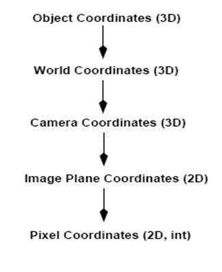
Thats how a 3d scene is transformed into 2d , with image of pixels.
Now we will explain this concept mathematically.
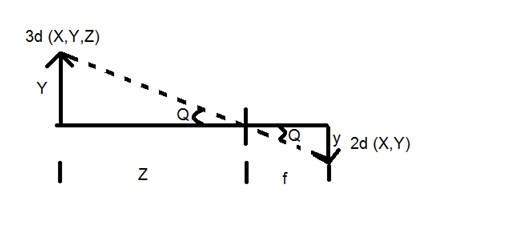 Where
Where
Y = 3d object
y = 2d Image
f = focal length of the camera
Z = distance between image and the camera
Now there are two different angles formed in this transform which are represented by Q.
The first angle is
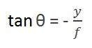
Where minus denotes that image is inverted. The second angle that is formed is:
Comparing these two equations we get
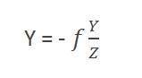
From this equation, we can see that when the rays of light reflect back after striking from the object , passed from the camera , an invert image is formed.
We can better understand this, with this example.
For example
Calculating the size of image formed
Suppose an image has been taken of a person 5m tall, and standing at a distance of 50m from the camera, and we have to tell that what is the size of the image of the person , with a camera of focal length is 50mm.
Solution:
Since the focal length is in millimeter , so we have to convert every thing in millimeter in order to calculate it.
So,
Y = 5000 mm.
f = 50 mm.
Z = 50000 mm.
Putting the values in the formula , we get
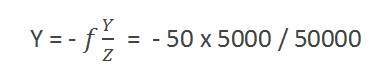
= -5 mm.
Again, the minus sign indicates that the image is inverted.
Concept of Bits Per Pixel
Bpp or bits per pixel denotes the number of bits per pixel. The number of different colors in an image is depends on the depth of color or bits per pixel.
Bits in mathematics:
Its just like playing with binary bits.
How many numbers can be represented by one bit.
0
1
How many two bits combinations can be made.
00
01
10
11
If we devise a formula for the calculation of total number of combinations that can be made from bit , it would be like this.
Where bpp denotes bits per pixel. Put 1 in the formula you get 2, put 2 in the formula , you get 4. It grows exponentionally.
Number of different colors:
Now as we said it in the beginning , that the number of different colors depend on the number of bits per pixel.
The table for some of the bits and their color is given below.
| Bits per pixel | Number of colors |
|---|---|
| 1 bpp | 2 colors |
| 2 bpp | 4 colors |
| 3 bpp | 8 colors |
| 4 bpp | 16 colors |
| 5 bpp | 32 colors |
| 6 bpp | 64 colors |
| 7 bpp | 128 colors |
| 8 bpp | 256 colors |
| 10 bpp | 1024 colors |
| 16 bpp | 65536 colors |
| 24 bpp | 16777216 colors (16.7 million colors) |
| 32 bpp | 4294967296 colors (4294 million colors) |
This table shows different bits per pixel and the amount of color they contain.
Shades
You can easily notice the pattern of the exponentional growth. The famous gray scale image is of 8 bpp , means it has 256 different colors in it or 256 shades.
Shades can be represented as:
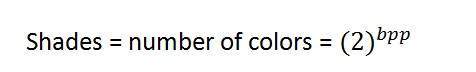
Color images are usually of the 24 bpp format , or 16 bpp.
We will see more about other color formats and image types in the tutorial of image types.
Color values:
We have previously seen in the tutorial of concept of pixel , that 0 pixel value denotes black color.Black color:
Remember , 0 pixel value always denotes black color. But there is no fixed value that denotes white color.White color:
The value that denotes white color can be calculated as :
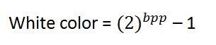
In case of 1 bpp , 0 denotes black , and 1 denotes white.
In case 8 bpp , 0 denotes black , and 255 denotes white.
Gray color:
When you calculate the black and white color value , then you can calculate the pixel value of gray color.
Gray color is actually the mid point of black and white. That said,
In case of 8bpp, the pixel value that denotes gray color is 127 or 128bpp (if you count from 1, not from 0).
Image storage requirements
After the discussion of bits per pixel , now we have every thing that we need to calculate a size of an image.
Image size
The size of an image depends upon three things.
Number of rows
Number of columns
Number of bits per pixel
The formula for calculating the size is given below.
Size of an image = rows * cols * bpp
It means that if you have an image, lets say this one:
Assuming it has 1024 rows and it has 1024 columns. And since it is a gray scale image , it has 256 different shades of gray or it has bits per pixel. Then putting these values in the formula , we get
Size of an image = rows * cols * bpp
= 1024 * 1024 * 8
= 8388608 bits.
But since its not a standard answer that we recognize , so will convert it into our format.
Converting it into bytes = 8388608 / 8 = 1048576 bytes.
Converting into kilo bytes = 1048576 / 1024 = 1024kb.
Converting into Mega bytes = 1024 / 1024 = 1 Mb.
Thats how an image size is calculated and it is stored. Now in the formula , if you are given the size of image and the bits per pixel , you can also calculate the rows and columns of the image , provided the image is square(same rows and same column).
Types of Images
There are many type of images , and we will look in detail about different types of images , and the color distribution in them.
The binary image
The binary image as it name states , contain only two pixel values.
0 and 1.
In our previous tutorial of bits per pixel , we have explained this in detail about the representation of pixel values to their respective colors.
Here 0 refers to black color and 1 refers to white color. It is also known as Monochrome.
Black and white image:
The resulting image that is formed hence consist of only black and white color and thus can also be called as Black and White image.
No gray level
One of the interesting this about this binary image that there is no gray level in it. Only two colors that are black and white are found in it.
Format
Binary images have a format of PBM ( Portable bit map )
2 , 3 , 4 ,5 ,6 bit color format
The images with a color format of 2 , 3 , 4 ,5 and 6 bit are not widely used today. They were used in old times for old TV displays , or monitor displays.
But each of these colors have more then two gray levels , and hence has gray color unlike the binary image.
In a 2 bit 4, in a 3 bit 8 , in a 4 bit 16, in a 5 bit 32, in a 6 bit 64 different colors are present.
8 bit color format
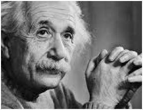
8 bit color format is one of the most famous image format. It has 256 different shades of colors in it. It is commonly known as Grayscale image.
The range of the colors in 8 bit vary from 0-255. Where 0 stands for black , and 255 stands for white , and 127 stands for gray color.
This format was used initially by early models of the operating systems UNIX and the early color Macintoshes.
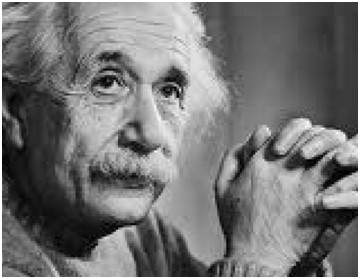
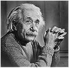
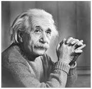
A grayscale image of Einstein is shown below:
Format
The format of these images are PGM ( Portable Gray Map ).
This format is not supported by default from windows. In order to see gray scale image , you need to have an image viewer or image processing toolbox such as Matlab.
Behind gray scale image:
As we have explained it several times in the previous tutorials , that an image is nothing but a two dimensional function , and can be represented by a two dimensional array or matrix. So in the case of the image of Einstein shown above , there would be two dimensional matrix in behind with values ranging between 0 and 255.
But thats not the case with the color images.
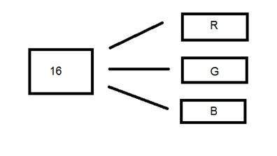
16 bit color format
It is a color image format. It has 65,536 different colors in it. It is also known as High color format.
It has been used by Microsoft in their systems that support more then 8 bit color format. Now in this 16 bit format and the next format we are going to discuss which is a 24 bit format are both color format.
The distribution of color in a color image is not as simple as it was in grayscale image.
A 16 bit format is actually divided into three further formats which are Red , Green and Blue. The famous (RGB) format.
It is pictorially represented in the image below.
Now the question arises , that how would you distribute 16 into three. If you do it like this,
5 bits for R , 5 bits for G , 5 bits for B
Then there is one bit remains in the end.
So the distribution of 16 bit has been done like this.
5 bits for R , 6 bits for G , 5 bits for B.
The additional bit that was left behind is added into the green bit. Because green is the color which is most soothing to eyes in all of these three colors.
Note this is distribution is not followed by all the systems. Some have introduced an alpha channel in the 16 bit.
Another distribution of 16 bit format is like this:
4 bits for R , 4 bits for G , 4 bits for B , 4 bits for alpha channel.
Or some distribute it like this
5 bits for R , 5 bits for G , 5 bits for B , 1 bits for alpha channel.
24 bit color format
24 bit color format also known as true color format. Like 16 bit color format , in a 24 bit color format , the 24 bits are again distributed in three different formats of Red , Green and Blue.
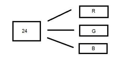
Since 24 is equally divided on 8 , so it has been distributed equally between three different color channels.
Their distribution is like this.
8 bits for R , 8 bits for G , 8 bits for B.
Behind a 24 bit image.
Unlike a 8 bit gray scale image , which has one matrix behind it, a 24 bit image has three different matrices of R , G , B.
Format
It is the most common used format. Its format is PPM ( Portable pixMap) which is supported by Linux operating system. The famous windows has its own format for it which is BMP ( Bitmap ).
Color Codes Conversion
In this tutorial , we will see that how different color codes can be combined to make other colors, and how we can covert RGB color codes to hex and vice versa.
Different color codes
All the colors here are of the 24 bit format, that means each color has 8 bits of red , 8 bits of green , 8 bits of blue , in it. Or we can say each color has three different portions. You just have to change the quantity of these three portions to make any color.
Binary color format
Color:Black
Image:
Decimal Code:
(0,0,0)
Explanation:
As it has been explained in the previous tutorials , that in an 8-bit format , 0 refers to black. So if we have to make a pure black color , we have to make all the three portion of R , G , B to 0.
Color:White
Image:

Decimal Code:
(255,255,255)
Explanation:
Since each portion of R,G,B is an 8 bit portion. So in 8-bit , the white color is formed by 255. It is explained in the tutorial of pixel. So in order to make a white color we set each portion to 255 and thats how we got a white color. By setting each of the value to 255 , we get overall value of 255 , thats make the color white.
RGB color model:
Color:Red
Image:

Decimal Code:
(255,0,0)
Explanation:
Since we need only red color , so we zero out the rest of the two portions which are green and blue , and we set the red portion to its maximum which is 255.
Color:Green
Image:

Decimal Code:
(0,255,0)
Explanation:
Since we need only green color , so we zero out the rest of the two portions which are red and blue , and we set the green portion to its maximum which is 255.
Color: Blue
Image:

Decimal Code:
(0,0,255)
Explanation:
Since we need only blue color , so we zero out the rest of the two portions which are red and green , and we set the blue portion to its maximum which is 255
Gray color:
Color: Gray
Image:

Decimal Code:
(128,128,128)
Explanation:
As we have already defined in our tutorial of pixel , that gray color Is actually the mid point. In an 8-bit format , the mid point is 128 or 127. In this case we choose 128. So we set each of the portion to its mid point which is 128 , and that results in overall mid value and we got gray color.
CMYK color model:
CMYK is another color model where c stands for cyan , m stands for magenta , y stands for yellow , and k for black. CMYK model is commonly used in color printers in which there are two carters of color is used. One consist of CMY and other consist of black color.
The colors of CMY can also made from changing the quantity or portion of red , green and blue.
Color: Cyan
Image:

Decimal Code:
(0,255,255)
Explanation:
Cyan color is formed from the combination of two different colors which are Green and blue. So we set those two to maximum and we zero out the portion of red. And we get cyan color.
Color: Magenta
Image:

Decimal Code:
(255,0,255)
Explanation:
Magenta color is formed from the combination of two different colors which are Red and Blue. So we set those two to maximum and we zero out the portion of green. And we get magenta color.
Color: Yellow
Image:

Decimal Code:
(255,255,0)
Explanation:
Yellow color is formed from the combination of two different colors which are Red and Green. So we set those two to maximum and we zero out the portion of blue. And we get yellow color.
Conversion
Now we will see that how color are converted are from one format to another.
Conversion from RGB to Hex code:
Conversion from Hex to rgb is done through this method:
Take a color. E.g: White = (255, 255 , 255).
Take the first portion e.g 255.
Divide it by 16. Like this:
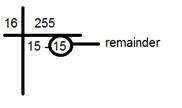
Take the two numbers below line , the factor , and the remainder. In this case it is 15 � 15 which is FF.
Repeat the step 2 for the next two portions.
Combine all the hex code into one.
Answer: #FFFFFF
Conversion from Hex to RGB:
Conversion from hex code to rgb decimal format is done in this way.
Take a hex number. E.g: #FFFFFF
Break this number into 3 parts: FF FF FF
Take the first part and separate its components: F F
Convert each of the part separately into binary: (1111) ( 1111)
Now combine the individual binaries into one: 11111111
Convert this binary into decimal: 255
Now repeat step 2 , two more times.
The value comes in the first step is R , second one is G, and the third one belongs to B.
Answer: ( 255 , 255 , 255 )
Common colors and their Hex code has been given in this table.
| Color | Hex Code |
|---|---|
| Black | #000000 |
| White | #FFFFFF |
| Gray | #808080 |
| Red | #FF0000 |
| Green | #00FF00 |
| Blue | #0000FF |
| Cyan | #00FFFF |
| Magenta | #FF00FF |
| Yellow | #FFFF00 |
Grayscael to RGB Conversion
We have already define the RGB color model and gray scale format in our tutorial of Image types. Now we will convert an color image into a grayscale image. There are two methods to convert it. Both has their own merits and demerits. The methods are:Average method
Weighted method or luminosity method
Average method
Average method is the most simple one. You just have to take the average of three colors. Since its an RGB image , so it means that you have add r with g with b and then divide it by 3 to get your desired grayscale image.
Its done in this way.
Grayscale = (R + G + B) / 3
For example:
If you have an color image like the image shown above and you want to convert it into grayscale using average method. The following result would appear.
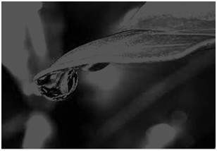
Explanation
There is one thing to be sure , that something happens to the original works. It means that our average method works. But the results were not as expected. We wanted to convert the image into a grayscale , but this turned out to be a rather black image.
Problem
This problem arise due to the fact , that we take average of the three colors. Since the three different colors have three different wavelength and have their own contribution in the formation of image , so we have to take average according to their contribution , not done it averagely using average method. Right now what we are doing is this,
33% of Red, 33% of Green, 33% of Blue
We are taking 33% of each, that means , each of the portion has same contribution in the image. But in reality thats not the case. The solution to this has been given by luminosity method.
Weighted method or luminosity method
You have seen the problem that occur in the average method. Weighted method has a solution to that problem. Since red color has more wavelength of all the three colors , and green is the color that has not only less wavelength then red color but also green is the color that gives more soothing effect to the eyes.
It means that we have to decrease the contribution of red color , and increase the contribution of the green color , and put blue color contribution in between these two.
So the new equation that form is:
New grayscale image = ( (0.3 * R) + (0.59 * G) + (0.11 * B) ).
According to this equation , Red has contribute 30% , Green has contributed 59% which is greater in all three colors and Blue has contributed 11%.
Applying this equation to the image, we get this
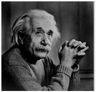
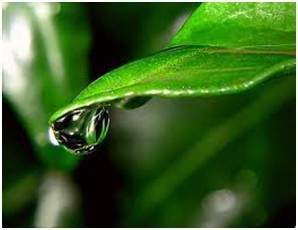
Original Image:
Grayscale Image:
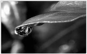
Explanation
As you can see here , that the image has now been properly converted to grayscale using weighted method. As compare to the result of average method , this image is more brighter.
Concept of Sampling
Conversion of analog signal to digital signal:
The output of most of the image sensors is an analog signal, and we can not apply digital processing on it because we can not store it. We can not store it because it requires infinite memory to store a signal that can have infinite values.
So we have to convert an analog signal into a digital signal.
To create an image which is digital , we need to covert continuous data into digital form. There are two steps in which it is done.
Sampling
Quantization
We will discuss sampling now , and quantization will be discussed later on but for now on we will discuss just a little about the difference between these two and the need of these two steps.
Basic idea:
The basic idea behind converting an analog signal to its digital signal is
to convert both of its axis (x,y) into a digital format.
Since an image is continuous not just in its co-ordinates (x axis) , but also in its amplitude (y axis), so the part that deals with the digitizing of co-ordinates is known as sampling. And the part that deals with digitizing the amplitude is known as quantization.
Sampling.
Sampling has already been introduced in our tutorial of introduction to signals and system. But we are going to discuss here more.
Here what we have discussed of the sampling.
The term sampling refers to take samples
We digitize x axis in sampling
It is done on independent variable
In case of equation y = sin(x), it is done on x variable
It is further divided into two parts , up sampling and down sampling
If you will look at the above figure , you will see that there are some random variations in the signal. These variations are due to noise. In sampling we reduce this noise by taking samples. It is obvious that more samples we take , the quality of the image would be more better, the noise would be more removed and same happens vice versa.
However , if you take sampling on the x axis , the signal is not converted to digital format , unless you take sampling of the y-axis too which is known as quantization. The more samples eventually means you are collecting more data, and in case of image , it means more pixels.
Relation ship with pixels
Since a pixel is a smallest element in an image. The total number of pixels in an image can be calculated as
Pixels = total no of rows * total no of columns.
Lets say we have total of 25 pixels , that means we have a square image of 5 X 5. Then as we have dicussed above in sampling , that more samples eventually result in more pixels. So it means that of our continuous signal , we have taken 25 samples on x axis. That refers to 25 pixels of this image.
This leads to another conclusion that since pixel is also the smallest division of a CCD array. So it means it has a relationship with CCD array too , which can be explained as this.
Relationship with CCD array
The number of sensors on a CCD array is directly equal to the number of pixels. And since we have concluded that the number of pixels is directly equal to the number of samples, that means that number sample is directly equal to the number of sensors on CCD array.
Oversampling.
In the beginning we have define that sampling is further categorize into two types. Which is up sampling and down sampling. Up sampling is also called as over sampling.
The oversampling has a very deep application in image processing which is known as Zooming.
Zooming
We will formally introduce zooming in the upcoming tutorial , but for now on , we will just briefly explain zooming.
Zooming refers to increase the quantity of pixels , so that when you zoom an image , you will see more detail.
The increase in the quantity of pixels is done through oversampling. The one way to zoom is , or to increase samples, is to zoom optically , through the motor movement of the lens and then capture the image. But we have to do it , once the image has been captured.
There is a difference between zooming and sampling.
The concept is same , which is, to increase samples. But the key difference is that while sampling is done on the signals , zooming is done on the digital image.
Pixel Resolution
Before we define pixel resolution, it is necessary to define a pixel.
Pixel
We have already defined a pixel in our tutorial of concept of pixel, in which we define a pixel as the smallest element of an image. We also defined that a pixel can store a value proportional to the light intensity at that particular location.
Now since we have defined a pixel, we are going to define what is resolution.
Resolution
The resolution can be defined in many ways. Such as pixel resolution , spatial resolution , temporal resolution , spectral resolution. Out of which we are going to discuss pixel resolution.
You have probably seen that in your own computer settings , you have monitor resolution of 800 x 600 , 640 x 480 e.t.c
In pixel resolution , the term resolution refers to the total number of count of pixels in an digital image. For example. If an image has M rows and N columns , then its resolution can be defined as M X N.
If we define resolution as the total number of pixels , then pixel resolution can be defined with set of two numbers. The first number the width of the picture , or the pixels across columns , and the second number is height of the picture , or the pixels across its width.
We can say that the higher is the pixel resolution , the higher is the quality of the image.
We can define pixel resolution of an image as 4500 X 5500.
Megapixels
We can calculate mega pixels of a camera using pixel resolution.
Column pixels (width ) X row pixels ( height ) / 1 Million.
The size of an image can be defined by its pixel resolution.
Size = pixel resolution X bpp ( bits per pixel )
Calculating the mega pixels of the camera
Lets say we have an image of dimension: 2500 X 3192.
Its pixel resolution = 2500 * 3192 = 7982350 bytes.
Dividing it by 1 million = 7.9 = 8 mega pixel (approximately).
Aspect ratio
Another important concept with the pixel resolution is aspect ratio.
Aspect ratio is the ratio between width of an image and the height of an image. It is commonly explained as two numbers separated by a colon (8:9). This ratio differs in different images , and in different screens. The common aspect ratios are:
1.33:1, 1.37:1, 1.43:1, 1.50:1, 1.56:1, 1.66:1, 1.75:1, 1.78:1, 1.85:1, 2.00:1, e.t.c
Advantage:
Aspect ratio maintains a balance between the appearance of an image on the screen , means it maintains a ratio between horizontal and vertical pixels. It does not let the image to get distorted when aspect ratio is increased.
For example:
This is a sample image , which has 100 rows and 100 columns. If we wish to make is smaller, and the condition is that the quality remains the same or in other way the image does not get distorted , here how it happens.
Original image:

Changing the rows and columns by maintain the aspect ratio in MS Paint.
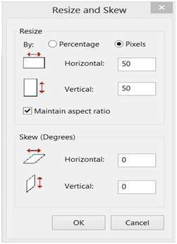
Result

Smaller image , but with same balance.
You have probably seen aspect ratios in the video players, where you can adjust the video according to your screen resolution.
Finding the dimensions of the image from aspect ratio:
Aspect ratio tells us many things. With the aspect ratio, you can calculate the dimensions of the image along with the size of the image.
For example
If you are given an image with aspect ratio of 6:2 of an image of pixel resolution of 480000 pixels given the image is an gray scale image.
And you are asked to calculate two things.
Resolve pixel resolution to calculate the dimensions of image
Calculate the size of the image
Solution:
Given:
Aspect ratio: c:r = 6:2
Pixel resolution: c * r = 480000
Bits per pixel: grayscale image = 8bpp
Find:
Number of rows = ?
Number of cols = ?
Solving first part:
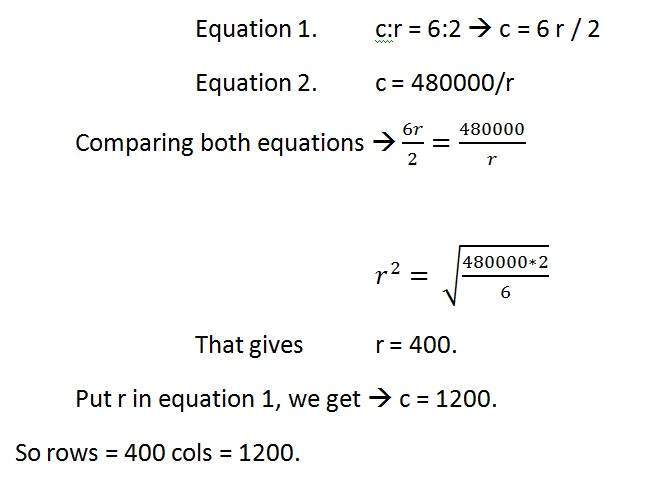
Solving 2nd part:
Size = rows * cols * bpp
Size of image in bits = 400 * 1200 * 8 = 3840000 bits
Size of image in bytes = 480000 bytes
Size of image in kilo bytes = 48 kb (approx).
Concept of Zooming
In this tutorial we are going to introduce the concept of zooming , and the common techniques that are used to zoom an image.
Zooming
Zooming simply means enlarging a picture in a sense that the details in the image became more visible and clear. Zooming an image has many wide applications ranging from zooming through a camera lens , to zoom an image on internet e.t.c.
For example
is zoomed into
You can zoom something at two different steps.
The first step includes zooming before taking an particular image. This is known as pre processing zoom. This zoom involves hardware and mechanical movement.
The second step is to zoom once an image has been captured. It is done through many different algorithms in which we manipulate pixels to zoom in the required portion.
We will discuss them in detail in the next tutorial.
Optical Zoom vs digital Zoom
These two types of zoom are supported by the cameras.
Optical Zoom:
The optical zoom is achieved using the movement of the lens of your camera. An optical zoom is actually a true zoom. The result of the optical zoom is far better then that of digital zoom. In optical zoom , an image is magnified by the lens in such a way that the objects in the image appear to be closer to the camera. In optical zoom the lens is physically extend to zoom or magnify an object.
Digital Zoom:
Digital zoom is basically image processing within a camera. During a digital zoom , the center of the image is magnified and the edges of the picture got crop out. Due to magnified center , it looks like that the object is closer to you.
During a digital zoom , the pixels got expand , due to which the quality of the image is compromised.
The same effect of digital zoom can be seen after the image is taken through your computer by using an image processing toolbox / software, such as Photoshop.
The following picture is the result of digital zoom done through one of the following methods given below in the zooming methods.

Now since we are leaning digital image processing , we will not focus , on how an image can be zoomed optically using lens or other stuff. Rather we will focus on the methods, that enable to zoom a digital image.
Zooming methods:
Although there are many methods that does this job , but we are going to discuss the most common of them here.
They are listed below.
Pixel replication or (Nearest neighbor interpolation)
Zero order hold method
Zooming K times
All these three methods are formally introduced in the next tutorial.
Zooming Methods
In this tutorial we are going to formally introduce three methods of zooming that were introduced in the tutorial of Introduction to zooming.
Methods
Pixel replication or (Nearest neighbor interpolation)
Zero order hold method
Zooming K times
Each of the methods have their own advantages and disadvantages. We will start by discussing pixel replication.
Method 1: Pixel replication:
Introduction:
It is also known as Nearest neighbor interpolation. As its name suggest , in this method , we just replicate the neighboring pixels. As we have already discussed in the tutorial of Sampling , that zooming is nothing but increase amount of sample or pixels. This algorithm works on the same principle.
Working:
In this method we create new pixels form the already given pixels. Each pixel is replicated in this method n times row wise and column wise and you got a zoomed image. Its as simple as that.
For example:
if you have an image of 2 rows and 2 columns and you want to zoom it twice or 2 times using pixel replication, here how it can be done.
For a better understanding , the image has been taken in the form of matrix with the pixel values of the image.
| 1 | 2 |
| 3 | 4 |
The above image has two rows and two columns, we will first zoom it row wise.
Row wise zooming:
When we zoom it row wise , we will just simple copy the rows pixels to its adjacent new cell.
Here how it would be done.
| 1 | 1 | 2 | 2 |
| 3 | 3 | 4 | 4 |
As you can that in the above matrix , each pixel is replicated twice in the rows.
Column size zooming:
The next step is to replicate each of the pixel column wise, that we will simply copy the column pixel to its adjacent new column or simply below it.
Here how it would be done.
| 1 | 1 | 2 | 2 |
| 1 | 1 | 2 | 2 |
| 3 | 3 | 4 | 4 |
| 3 | 3 | 4 | 4 |
New image size:
As it can be seen from the above example , that an original image of 2 rows and 2 columns has been converted into 4 rows and 4 columns after zooming. That means the new image has a dimensions of
(Original image rows * zooming factor, Original Image cols * zooming factor)
Advantage and disadvantage:
One of the advantage of this zooming technique is , it is very simple. You just have to copy the pixels and nothing else.
The disadvantage of this technique is that image got zoomed but the output is very blurry. And as the zooming factor increased , the image got more and more blurred. That would eventually result in fully blurred image.
Method 2: Zero order hold
Introduction
Zero order hold method is another method of zooming. It is also known as zoom twice. Because it can only zoom twice. We will see in the below example that why it does that.
Working
In zero order hold method , we pick two adjacent elements from the rows respectively and then we add them and divide the result by two, and place their result in between those two elements. We first do this row wise and then we do this column wise.
For example
Lets take an image of the dimensions of 2 rows and 2 columns and zoom it twice using zero order hold.
| 1 | 2 |
| 3 | 4 |
First we will zoom it row wise and then column wise.
Row wise zooming
| 1 | 1 | 2 |
| 3 | 3 | 4 |
As we take the first two numbers : (2 + 1) = 3 and then we divide it by 2, we get 1.5 which is approximated to 1. The same method is applied in the row 2.
Column wise zooming
| 1 | 1 | 2 |
| 2 | 2 | 3 |
| 3 | 3 | 4 |
We take two adjacent column pixel values which are 1 and 3. We add them and got 4. 4 is then divided by 2 and we get 2 which is placed in between them. The same method is applied in all the columns.
New image size
As you can see that the dimensions of the new image are 3 x 3 where the original image dimensions are 2 x 2. So it means that the dimensions of the new image are based on the following formula
(2(number of rows) minus 1) X (2(number of columns) minus 1)
Advantages and disadvantage.
One of the advantage of this zooming technique , that it does not create as blurry picture as compare to the nearest neighbor interpolation method. But it also has a disadvantage that it can only run on the power of 2. It can be demonstrated here.
Reason behind twice zooming:
Consider the above image of 2 rows and 2 columns. If we have to zoom it 6 times , using zero order hold method , we can not do it. As the formula shows us this.
It could only zoom in the power of 2 2,4,8,16,32 and so on.
Even if you try to zoom it, you can not. Because at first when you will zoom it two times, and the result would be same as shown in the column wise zooming with dimensions equal to 3x3. Then you will zoom it again and you will get dimensions equal to 5 x 5. Now if you will do it again, you will get dimensions equal to 9 x 9.
Whereas according to the formula of yours the answer should be 11x11. As (6(2) minus 1) X (6(2) minus 1) gives 11 x 11.
Method 3: K-Times zooming
Introduction:
K times is the third zooming method we are going to discuss. It is one of the most perfect zooming algorithm discussed so far. It caters the challenges of both twice zooming and pixel replication. K in this zooming algorithm stands for zooming factor.
Working:
It works like this way.
First of all , you have to take two adjacent pixels as you did in the zooming twice. Then you have to subtract the smaller from the greater one. We call this output (OP).
Divide the output(OP) with the zooming factor(K). Now you have to add the result to the smaller value and put the result in between those two values.
Add the value OP again to the value you just put and place it again next to the previous putted value. You have to do it till you place k-1 values in it.
Repeat the same step for all the rows and the columns , and you get a zoomed images.
For example:
Suppose you have an image of 2 rows and 3 columns , which is given below. And you have to zoom it thrice or three times.
| 15 | 30 | 15 |
| 30 | 15 | 30 |
K in this case is 3. K = 3.
The number of values that should be inserted is k-1 = 3-1 = 2.
Row wise zooming
Take the first two adjacent pixels. Which are 15 and 30.
Subtract 15 from 30. 30-15 = 15.
Divide 15 by k. 15/k = 15/3 = 5. We call it OP.(where op is just a name)
Add OP to lower number. 15 + OP = 15 + 5 = 20.
Add OP to 20 again. 20 + OP = 20 + 5 = 25.
We do that 2 times because we have to insert k-1 values.
Now repeat this step for the next two adjacent pixels. It is shown in the first table.
After inserting the values , you have to sort the inserted values in ascending order, so there remains a symmetry between them.
It is shown in the second table
Table 1.
| 15 | 20 | 25 | 30 | 20 | 25 | 15 |
| 30 | 20 | 25 | 15 | 20 | 25 | 30 |
Table 2.
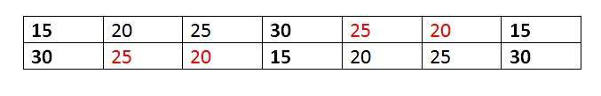
Column wise zooming
The same procedure has to be performed column wise. The procedure include taking the two adjacent pixel values, and then subtracting the smaller from the bigger one. Then after that , you have to divide it by k. Store the result as OP. Add OP to smaller one, and then again add OP to the value that comes in first addition of OP. Insert the new values.
Here what you got after all that.
| 15 | 20 | 25 | 30 | 25 | 20 | 15 |
| 20 | 21 | 21 | 25 | 21 | 21 | 20 |
| 25 | 22 | 22 | 20 | 22 | 22 | 25 |
| 30 | 25 | 20 | 15 | 20 | 25 | 30 |
New image size
The best way to calculate the formula for the dimensions of a new image is to compare the dimensions of the original image and the final image. The dimensions of the original image were 2 X 3. And the dimensions of the new image are 4 x 7.
The formula thus is:
(K (number of rows minus 1) + 1) X (K (number of cols minus 1) + 1)
Advantages and disadvantages
The one of the clear advantage that k time zooming algorithm has that it is able to compute zoom of any factor which was the power of pixel replication algorithm , also it gives improved result (less blurry) which was the power of zero order hold method. So hence It comprises the power of the two algorithms.
The only difficulty this algorithm has that it has to be sort in the end , which is an additional step , and thus increases the cost of computation.
Spatial Resolution
Image resolution
Image resolution can be defined in many ways. One type of it which is pixel resolution that has been discussed in the tutorial of pixel resolution and aspect ratio.
In this tutorial, we are going to define another type of resolution which is spatial resolution.
Spatial resolution:
Spatial resolution states that the clarity of an image cannot be determined by the pixel resolution. The number of pixels in an image does not matter.
Spatial resolution can be defined as the
smallest discernible detail in an image. (Digital Image Processing - Gonzalez, Woods - 2nd Edition)
Or in other way we can define spatial resolution as the number of independent pixels values per inch.
In short what spatial resolution refers to is that we cannot compare two different types of images to see that which one is clear or which one is not. If we have to compare the two images , to see which one is more clear or which has more spatial resolution , we have to compare two images of the same size.
For example:
You cannot compare these two images to see the clarity of the image.
Although both images are of the same person , but that is not the condition we are judging on. The picture on the left is zoomed out picture of Einstein with dimensions of 227 x 222. Whereas the picture on the right side has the dimensions of 980 X 749 and also it is a zoomed image. We cannot compare them to see that which one is more clear. Remember the factor of zoom does not matter in this condition, the only thing that matters is that these two pictures are not equal.
So in order to measure spatial resolution , the pictures below would server the purpose.
Now you can compare these two pictures. Both the pictures has same dimensions which are of 227 X 222. Now when you compare them , you will see that the picture on the left side has more spatial resolution or it is more clear then the picture on the right side. That is because the picture on the right is a blurred image.
Measuring spatial resolution:
Since the spatial resolution refers to clarity , so for different devices , different measure has been made to measure it.
For example:
Dots per inch
Lines per inch
Pixels per inch
They are discussed in more detail in the next tutorial but just a brief introduction has been given below.
Dots per inch:
Dots per inch or DPI is usually used in monitors.
Lines per inch:
Lines per inch or LPI is usually used in laser printers.
Pixel per inch:
Pixel per inch or PPI is measure for different devices such as tablets , Mobile phones e.t.c.
Pixels,Dots and Lines Per Inch
In the previous tutorial of spatial resolution , we discussed the brief introduction of PPI, DPI, LPI. Now we are formally going to discuss all of them.
Pixels per inch.
Pixel density or Pixels per inch is a measure of spatial resolution for different devices that includes tablets , mobile phones.
The higher is the PPI , the higher is the quality. In order to more understand it, that how it calculated. Lets calculate the PPI of a mobile phone.
Calculating pixels per inch (PPI) of Samsung galaxy S4:

The Samsung galaxy s4 has PPI or pixel density of 441. But how does it is calculated?
First of all we will Pythagoras theorem to calculate the diagonal resolution in pixels.
It can be given as:
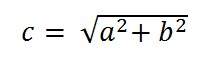
Where a and b are the height and width resolutions in pixel and c is the diagonal resolution in pixels.
For Samsung galaxy s4 , it is 1080 x 1920 pixels.
So putting those values in the equation gives the result
C = 2202.90717
Now we will calculate PPI
PPI = c / diagonal size in inches
The diagonal size in inches of Samsun galaxy s4 is 5.0 inches , which can be confirmed from anywhere.
PPI = 2202.90717/5.0
PPI = 440.58
PPI = 441 (approx)
That means that the pixel density of Samsung galaxy s4 is 441 PPI.
Dots per inch.
The dpi is often relate to PPI , whereas there is a difference between these two. DPI or dots per inch is a measure of spatial resolution of printers. In case of printers , dpi means that how many dots of ink are printed per inch when an image get printed out from the printer.
Remember , it is not necessary that each Pixel per inch is printed by one dot per inch. There may be many dots per inch used for printing one pixel. The reason behind this that most of the color printers uses CMYK model. The colors are limited. Printer has to choose from these colors to make the color of the pixel whereas within pc , you have hundreds of thousands of colors.
The higher is the dpi of the printer , the higher is the quality of the printed document or image on paper.
Usually some of the laser printers have dpi of 300 and some have 600 or more.
Lines per inch.
When dpi refers to dots per inch, liner per inch refers to lines of dots per inch. The resolution of halftone screen is measured in lines per inch.
The following table shows some of the lines per inch capacity of the printers.
| Printer | LPI |
|---|---|
| Screen printing | 45-65 lpi |
| Laser printer (300 dpi) | 65 lpi |
| Laser printer (600 dpi) | 85-105 lpi |
| Offset Press (newsprint paper) | 85 lpi |
| Offset Press (coated paper) | 85-185 lpi |
Gray Level Resolution
Image resolution:
A resolution can be defined as the total number of pixels in an image. This has been discussed in Image resolution. And we have also discussed, that clarity of an image doesnot depends on number of pixels, but on the spatial resolution of the image. This has been discussed in the spatial resolution. Here we are going to discuss another type of resolution which is called gray level resolution.Gray level resolution:
Gray level resolution refers to the predictable or deterministic change in the shades or levels of gray in an image.
In short gray level resolution is equal to the number of bits per pixel.
We have already discussed bits per pixel in our tutorial of bits per pixel and image storage requirements. We will define bpp here briefly.
BPP:
The number of different colors in an image is depends on the depth of color or bits per pixel.
Mathematically:
The mathematical relation that can be established between gray level resolution and bits per pixel can be given as.
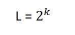
In this equation L refers to number of gray levels. It can also be defined as the shades of gray. And k refers to bpp or bits per pixel. So the 2 raise to the power of bits per pixel is equal to the gray level resolution.
For example:
The above image of Einstein is an gray scale image. Means it is an image with 8 bits per pixel or 8bpp.
Now if were to calculate the gray level resolution, here how we gonna do it.
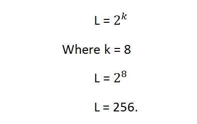
It means it gray level resolution is 256. Or in other way we can say that this image has 256 different shades of gray.
The more is the bits per pixel of an image , the more is its gray level resolution.
Defining gray level resolution in terms of bpp:
It is not necessary that a gray level resolution should only be defined in terms of levels. We can also define it in terms of bits per pixel.
For example:
If you are given an image of 4 bpp , and you are asked to calculate its gray level resolution. There are two answers to that question.
The first answer is 16 levels.
The second answer is 4 bits.
Finding bpp from Gray level resolution:
You can also find the bits per pixels from the given gray level resolution. For this , we just have to twist the formula a little.
Equation 1.
This formula finds the levels. Now if we were to find the bits per pixel or in this case k, we will simply change it like this.
K = log base 2(L) Equation (2)
Because in the first equation the relationship between Levels (L ) and bits per pixel (k) is exponentional. Now we have to revert it , and thus the inverse of exponentional is log.
Lets take an example to find bits per pixel from gray level resolution.
For example:
If you are given an image of 256 levels. What is the bits per pixel required for it.
Putting 256 in the equation , we get.
K = log base 2 ( 256)
K = 8.
So the answer is 8 bits per pixel.
Gray level resolution and quantization:
The quantization will be formally introduced in the next tutorial , but here we are just going to explain the relation ship between gray level resolution and quantization.
Gray level resolution is found on the y axis of the signal. In the tutorial of Introduction to signals and system , we have studied that digitizing a an analog signal requires two steps. Sampling and quantization.
Sampling is done on x axis. And quantization is done in Y axis.
So that means digitizing the gray level resolution of an image is done in quantization.
Concept of Quantization
We have introduced quantization in our tutorial of signals and system. We are formally going to relate it with digital images in this tutorial. Lets discuss first a little bit about quantization.
Digitizing a signal.
As we have seen in the previous tutorials , that digitizing an analog signal into a digital , requires two basic steps. Sampling and quantization. Sampling is done on x axis. It is the conversion of x axis (infinite values) to digital values.
The below figure shows sampling of a signal.
Sampling with relation to digital images:
The concept of sampling is directly related to zooming. The more samples you take , the more pixels , you get. Oversampling can also be called as zooming. This has been discussed under sampling and zooming tutorial.
But the story of digitizing a signal does not end at sampling too, there is another step involved which is known as Quantization.
What is quantization.
Quantization is opposite to sampling. It is done on y axis. When you are qunaitizing an image , you are actually dividing a signal into quanta(partitions).
On the x axis of the signal , are the co-ordinate values, and on the y axis , we have amplitudes. So digitizing the amplitudes is known as Quantization.
Here how it is done
You can see in this image , that the signal has been quantified into three different levels. That means that when we sample an image , we actually gather a lot of values, and in quantization , we set levels to these values. This can be more clear in the image below.
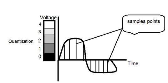
In the figure shown in sampling , although the samples has been taken , but they were still spanning vertically to a continuous range of gray level values. In the figure shown above , these vertically ranging values have been quantized into 5 different levels or partitions. Ranging from 0 black to 4 white. This level could vary according to the type of image you want.
The relation of quantization with gray levels has been further discussed below.
Relation of Quantization with gray level resolution:
The quantized figure shown above has 5 different levels of gray. It means that the image formed from this signal , would only have 5 different colors. It would be a black and white image more or less with some colors of gray. Now if you were to make the quality of the image more better, there is one thing you can do here. Which is , to increase the levels , or gray level resolution up. If you increase this level to 256, it means you have an gray scale image. Which is far better then simple black and white image.
Now 256 , or 5 or what ever level you choose is called gray level. Remember the formula that we discussed in the previous tutorial of gray level resolution which is,
We have discussed that gray level can be defined in two ways. Which were these two.
Gray level = number of bits per pixel (BPP).(k in the equation)
Gray level = number of levels per pixel.
In this case we have gray level is equal to 256. If we have to calculate the number of bits , we would simply put the values in the equation. In case of 256levels , we have 256 different shades of gray and 8 bits per pixel, hence the image would be a gray scale image.
Reducing the gray level
Now we will reduce the gray levels of the image to see the effect on the image.
For example:
Lets say you have an image of 8bpp, that has 256 different levels. It is a grayscale image and the image looks something like this.
256 Gray Levels
Now we will start reducing the gray levels. We will first reduce the gray levels from 256 to 128.
128 Gray Levels
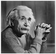
There is not much effect on an image after decrease the gray levels to its half. Lets decrease some more.
64 Gray Levels
Still not much effect , then lets reduce the levels more.
32 Gray Levels

Surprised to see , that there is still some little effect . May be its due to reason , that it is the picture of Einstein , but lets reduce the levels more.
16 Gray Levels
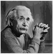
Boom here , we go , the image finally reveals , that it is effected by the levels.
8 Gray Levels
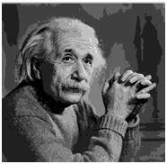
4 Gray Levels
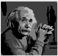
Now before reducing it , further two 2 levels , you can easily see that the image has been distorted badly by reducing the gray levels. Now we will reduce it to 2 levels, which is nothing but a simple black and white level. It means the image would be simple black and white image.
2 Gray Levels
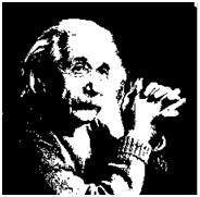
Thats the last level we can achieve , because if reduce it further , it would be simply a black image , which can not be interpreted.
Contouring:
There is an interesting observation here , that as we reduce the number of gray levels , there is a special type of effect start appearing in the image , which can be seen clear in 16 gray level picture. This effect is known as Contouring.
Iso preference curves:
The answer to this effect , that why it appears , lies in Iso preference curves. They are discussed in our next tutorial of Contouring and Iso preference curves.
ISO preference curves
What is contouring?
As we decrease the number of gray levels in an image , some false colors , or edges start appearing on an image. This has been shown in our last tutorial of Quantization.
Lets have a look at it.
Consider we , have an image of 8bpp (a grayscale image) with 256 different shades of gray or gray levels.
This above picture has 256 different shades of gray. Now when we reduce it to 128 and further reduce it 64, the image is more or less the same. But when re reduce it further to 32 different levels , we got a picture like this
If you will look closely , you will find that the effects start appearing on the image.These effects are more visible when we reduce it further to 16 levels and we got an image like this.
These lines, that start appearing on this image are known as contouring that are very much visible in the above image.
Increase and decrease in contouring
The effect of contouring increase as we reduce the number of gray levels and the effect decrease as we increase the number of gray levels. They are both vice versa
VS
That means more quantization , will effect in more contouring and vice versa. But is this always the case. The answer is No. That depends on something else that is discussed below.
Isopreference curves
A study conducted on this effect of gray level and contouring , and the results were shown in the graph in the form of curves , known as Iso preference curves.
The phenomena of Isopreference curves shows , that the effect of contouring not only depends on the decreasing of gray level resolution but also on the image detail.
The essence of the study is:
If an image has more detail , the effect of contouring would start appear on this image later, as compare to an image which has less detail, when the gray levels are quantized.
According to the original research, the researchers took these three images and they vary the Gray level resolution , in all three images.
The images were
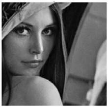
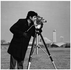
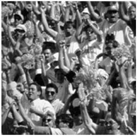
Level of detail:
The first image has only a face in it, and hence very less detail. The second image has some other objects in the image too , such as camera man, his camera , camera stand, and background objects e.t.c. Whereas the third image has more details then all the other images.
Experiment:
The gray level resolution was varied in all the images , and the audience was asked to rate these three images subjectively. After the rating , a graph was drawn according to the results.
Result:
The result was drawn on the graph. Each curve on the graph represents one image. The values on the x axis represents the number of gray levels and the values on the y axis represents bits per pixel (k).
The graph has been shown below.
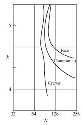
According to this graph , we can see that the first image which was of face , was subject to contouring early then all of the other two images. The second image , that was of the cameraman was subject to contouring a bit after the first image when its gray levels are reduced. This is because it has more details then the first image. And the third image was subject to contouring a lot after the first two images i-e: after 4 bpp. This is because , this image has more details.
Conclusion:
So for more detailed images, the isopreference curves become more and more vertical. It also means that for an image with a large amount of details , very few gray levels are needed.
Concept of Dithering
In the last two tutorials of Quantization and contouring , we have seen that reducing the gray level of an image reduces the number of colors required to denote an image. If the gray levels are reduced two 2 , the image that appears doesnot have much spatial resolution or is not very much appealing.
Dithering:
Dithering is the process by which we create illusions of the color that are not present actually. It is done by the random arrangement of pixels.
For example. Consider this image.
This is an image with only black and white pixels in it. Its pixels are arranged in an order to form another image that is shown below. Note at the arrangement of pixels has been changed , but not the quantity of pixels.
Why Dithering?
Why do we need dithering , the answer of this lies in its relation with quantization.
Dithering with quantization.
When we perform quantization , to the last level , we see that the image that comes in the last level (level 2) looks like this.
Now as we can see from the image here , that the picture is not very clear, especially if you will look at the left arm and back of the image of the Einstein. Also this picture does not have much information or detail of the Einstein.
Now if we were to change this image into some image that gives more detail then this, we have to perform dithering.
Performing dithering.
First of all , we will work on threholding. Dithering is usually working to improve thresholding. During threholding, the sharp edges appear where gradients are smooth in an image.
In thresholding , we simply choose a constant value. All the pixels above that value are considered as 1 and all the value below it are considered as 0.
We got this image after thresholding.
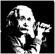
Since there is not much change in the image , as the values are already 0 and 1 or black and white in this image.
Now we perform some random dithering to it. Its some random arrangement of pixels.
We got an image that gives slighter of the more details , but its contrast is very low.
So we do some more dithering that will increase the contrast. The image that we got is this:
Now we mix the concepts of random dithering , along with threshold and we got an image like this.
Now you see , we got all these images by just re-arranging the pixels of an image. This re-arranging could be random or could be according to some measure.
Histograms Introduction
Before discussing the use of Histograms in image processing , we will first look at what histogram is, how it is used and then an example of histograms to have more understanding of histogram.
Histograms:
A histogram is a graph. A graph that shows frequency of anything. Usually histogram have bars that represent frequency of occurring of data in the whole data set.
A Histogram has two axis the x axis and the y axis.
The x axis contains event whose frequency you have to count.
The y axis contains frequency.
The different heights of bar shows different frequency of occurrence of data.
Usually a histogram looks like this.
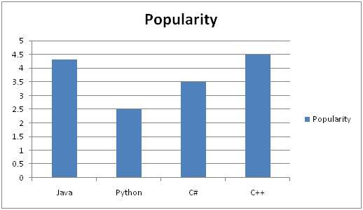
Now we will see an example of this histogram is build
Example:
Consider a class of programming students and you are teaching python to them.
At the end of the semester , you got this result that is shown in table. But it is very messy and doesnot show your overall result of class. So you have to make a histogram of your result , showing the overall frequency of occurrence of grades in your class. Here how you are going to do it.
Result sheet:
| Name | Grade |
|---|---|
| John | A |
| Jack | D |
| Carter | B |
| Tommy | A |
| Lisa | C+ |
| Derek | A- |
| Tom | B+ |
Histogram of result sheet:
Now what you are going to do is, that you have to find what comes on the x and the y axis.
There is one thing to be sure, that y axis contains the frequency, so what comes on the x axis. X axis contains the event whose frequency has to be calculated. In this case x axis contains grades.
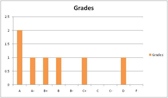
Now we will how do we use a histogram in an image.
Histogram of an image
Histogram of an image , like other histograms also shows frequency. But an image histogram , shows frequency of pixels intensity values. In an image histogram, the x axis shows the gray level intensities and the y axis shows the frequency of these intensities.
For example:
The histogram of the above picture of the Einstein would be something like this
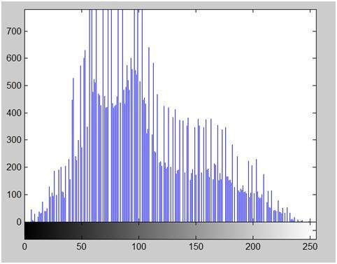
The x axis of the histogram shows the range of pixel values. Since its an 8 bpp image , that means it has 256 levels of gray or shades of gray in it. Thats why the range of x axis starts from 0 and end at 255 with a gap of 50. Whereas on the y axis , is the count of these intensities.
As you can see from the graph , that most of the bars that have high frequency lies in the first half portion which is the darker portion. That means that the image we have got is darker. And this can be proved from the image too.
Applications of Histograms:
Histograms has many uses in image processing. The first use as it has also been discussed above is the analysis of the image. We can predict about an image by just looking at its histogram. Its like looking an x ray of a bone of a body.
The second use of histogram is for brightness purposes. The histograms has wide application in image brightness. Not only in brightness , but histograms are also used in adjusting contrast of an image.
Another important use of histogram is to equalize an image.
And last but not the least, histogram has wide use in thresholding. This is mostly used in computer vision.
Brightness and Contrast
Brightness:
Brightness is a relative term. It depends on your visual perception. Since brightness is a relative term , so brightness can be defined as the amount of energy output by a source of light relative to the source we are comparing it to. In some cases we can easily say that the image is bright , and in some cases, its not easy to perceive.
For example:
Just have a look at both of these images , and compare which one is brighter.
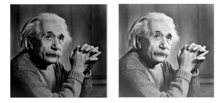
We can easily see , that the image on the right side is brighter as compared to the image on the left.
But if the image on the right is made more darker then the first one , then we can say that the image on the left is more brighter then the left.
How to make an image brighter.
Brightness can be simply increased or decreased by simple addition or subtraction, to the image matrix.
Consider this black image of 5 rows and 5 columns

Since we already know, that each image has a matrix at its behind that contains the pixel values. This image matrix is given below.
| 0 | 0 | 0 | 0 | 0 |
| 0 | 0 | 0 | 0 | 0 |
| 0 | 0 | 0 | 0 | 0 |
| 0 | 0 | 0 | 0 | 0 |
| 0 | 0 | 0 | 0 | 0 |
Since the whole matrix is filled with zero, and the image is very much darker.
Now we will compare it with another same black image to see this image got brighter or not.
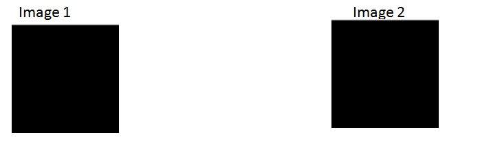
Still, both images look the same. To make the second one brighter we just need to add the value 1 to each element in the matrix representing it.
What we will do is , that we will simply add a value of 1 to each of the matrix value of image 1. After adding the image 1 would something like this.
Now we will again compare it with image 2 , and see any difference.
We see, that still we cannot tell which image is brighter as both images looks the same.
Now what we will do , is that we will add 50 to each of the matrix value of the image 1 and see what the image has become.
The output is given below.

Now again , we will compare it with image 2.
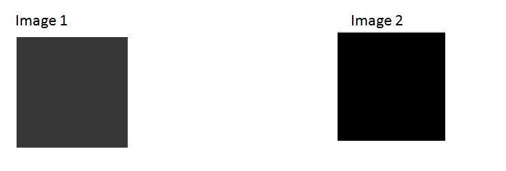
Now you can see that the image 1 is slightly brighter then the image 2. We go on , and add another 45 value to its matrix of image 1 , and this time we compare again both images.
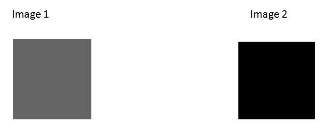
Now when you compare it , you can see that this image1 is clearly brighter then the image 2.
Even it is brighter then the old image1. At this point the matrix of the image1 contains 100 at each index as first add 5 , then 50 , then 45. So 5 + 50 + 45 = 100.
Contrast
Contrast can be simply explained as the difference between maximum and minimum pixel intensity in an image.
For example.
Consider the final image1 in brightness.

The matrix of this image is:
| 100 | 100 | 100 | 100 | 100 |
| 100 | 100 | 100 | 100 | 100 |
| 100 | 100 | 100 | 100 | 100 |
| 100 | 100 | 100 | 100 | 100 |
| 100 | 100 | 100 | 100 | 100 |
The maximum value in this matrix is 100.
The minimum value in this matrix is 100.
Contrast = maximum pixel intensity(subtracted by) minimum pixel intensity
= 100 (subtracted by) 100
= 0
0 means that this image has 0 contrast.
Image Transformations
Before we discuss, what is image transformation, we will discuss what a transformation is.
Transformation.
Transformation is a function. A function that maps one set to another set after performing some operations.
Digital Image Processing system:
We have already seen in the introductory tutorials that in digital image processing , we will develop a system that whose input would be an image and output would be an image too. And the system would perform some processing on the input image and gives its output as an processed image. It is shown below.
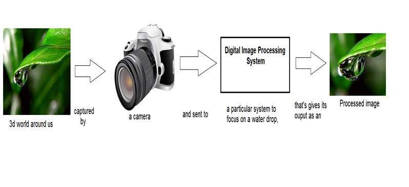
Now function applied inside this digital system that process an image and convert it into output can be called as transformation function.
As it shows transformation or relation , that how an image1 is converted to image2.
Image transformation.
Consider this equation
G(x,y) = T{ f(x,y) }
In this equation ,
F(x,y) = input image on which transformation function has to be applied.
G(x,y) = the output image or processed image.
T is the transformation function.
This relation between input image and the processed output image can also be represented as.
s = T (r)
where r is actually the pixel value or gray level intensity of f(x,y) at any point. And s is the pixel value or gray level intensity of g(x,y) at any point.
The basic gray level transformation has been discussed in our tutorial of basic gray level transformations.
Now we are going to discuss some of the very basic transformation functions.
Examples:
Consider this transformation function.
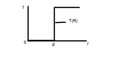
Lets take the point r to be 256, and the point p to be 127. Consider this image to be a one bpp image. That means we have only two levels of intensities that are 0 and 1. So in this case the transformation shown by the graph can be explained as.
All the pixel intensity values that are below 127 (point p) are 0 , means black. And all the pixel intensity values that are greater then 127, are 1 , that means white. But at the exact point of 127, there is a sudden change in transmission, so we cannot tell that at that exact point , the value would be 0 or 1.
Mathematically this transformation function can be denoted as:
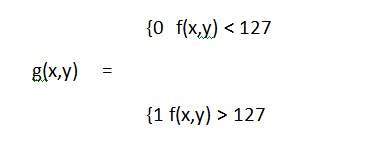
Consider another transformation like this:
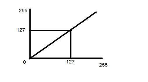
Now if you will look at this particular graph , you will see a straight transition line between input image and output image.
It shows that for each pixel or intensity value of input image, there is a same intensity value of output image. That means the output image is exact replica of the input image.
It can be mathematically represented as:
g(x,y) = f(x,y)
the input and output image would be in this case are shown below.
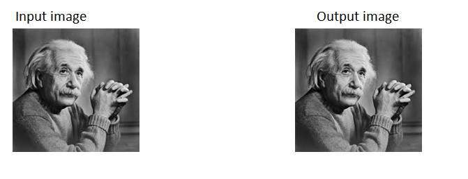
Histogram Sliding
The basic concept of histograms has been discussed in the tutorial of Introduction to histograms. But we will briefly introduce the histogram here.
Histogram:
Histogram is nothing but a graph that shows frequency of occurrence of data. Histograms has many use in image processing, out of which we are going to discuss one user here which is called histogram sliding.
Histogram sliding.
In histogram sliding , we just simply shift a complete histogram rightwards or leftwards. Due to shifting or sliding of histogram towards right or left , a clear change can be seen in the image.In this tutorial we are going to use histogram sliding for manipulating brightness.
The term i-e: Brightness has been discussed in our tutorial of introduction to brightness and contrast. But we are going to briefly define here.
Brightness:
Brightness is a relative term. Brightness can be defined as intensity of light emit by a particular light source.
Contrast:
Contrast can be defined as the difference between maximum and minimum pixel intensity in an image.
Sliding Histograms
Increasing brightness using histogram sliding
Histogram of this image has been shown below.
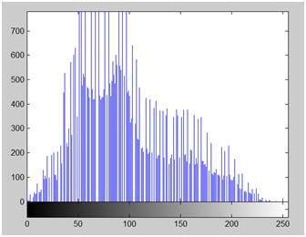
On the y axis of this histogram are the frequency or count. And on the x axis , we have gray level values. As you can see from the above histogram , that those gray level intensities whose count is more then 700, lies in the first half portion, means towards blacker portion. Thats why we got an image that is a bit darker.
In order to bright it, we will slide its histogram towards right , or towards whiter portion. In order to do we need to add atleast a value of 50 to this image. Because we can see from the histogram above , that this image also has 0 pixel intensities , that are pure black. So if we add 0 to 50 , we will shift all the values lies at 0 intensity to 50 intensity and all the rest of the values will be shifted accordingly.
Lets do it.
Here what we got after adding 50 to each pixel intensity.
The image has been shown below.
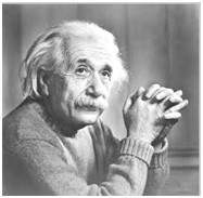
And its histogram has been shown below.
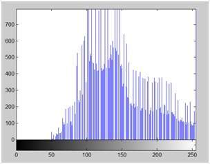
Lets compare these two images and their histograms to see that what change have to got.
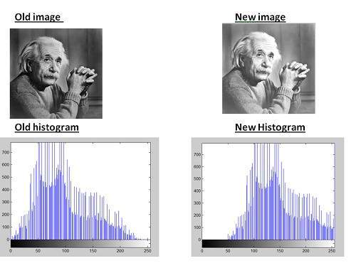
Conclusion:
As we can clearly see from the new histogram that all the pixels values has been shifted towards right and its effect can be seen in the new image.
Decreasing brightness using histogram sliding
Now if we were to decrease brightness of this new image to such an extent that the old image look brighter , we got to subtract some value from all the matrix of the new image. The value which we are going to subtract is 80. Because we already add 50 to the original image and we got a new brighter image, now if we want to make it darker , we have to subtract at least more than 50 from it.
And this what we got after subtracting 80 from the new image.
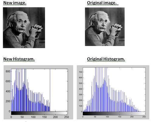
Conclusion:
It is clear from the histogram of the new image , that all the pixel values has been shifted towards right and thus , it can be validated from the image that new image is darker and now the original image look brighter as compare to this new image.
Histogram stretching
One of the other advantage of Histogram s that we discussed in our tutorial of introduction to histograms is contrast enhancement.
There are two methods of enhancing contrast. The first one is called Histogram stretching that increase contrast. The second one is called Histogram equalization that enhance contrast and it has been discussed in our tutorial of histogram equalization.
Before we will discuss the histogram stretching to increase contrast , we will briefly define contrast.
Contrast.
Contrast is the difference between maximum and minimum pixel intensity.
Consider this image.
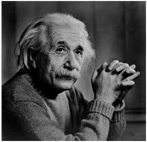
The histogram of this image is shown below.
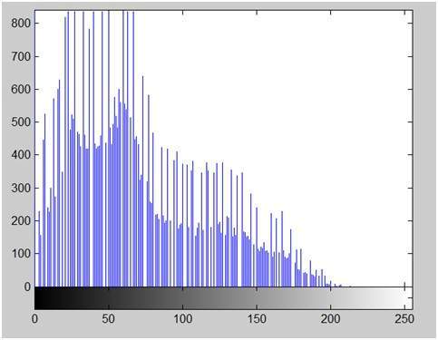
Now we calculate contrast from this image.
Contrast = 225.
Now we will increase the contrast of the image.
Increasing the contrast of the image:
The formula for stretching the histogram of the image to increase the contrast is
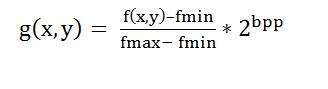
The formula requires finding the minimum and maximum pixel intensity multiply by levels of gray. In our case the image is 8bpp, so levels of gray are 256.
The minimum value is 0 and the maximum value is 225. So the formula in our case is
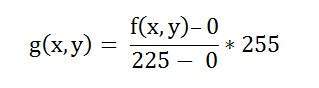
where f(x,y) denotes the value of each pixel intensity. For each f(x,y) in an image , we will calculate this formula.
After doing this, we will be able to enhance our contrast.
The following image appear after applying histogram stretching.

The stretched histogram of this image has been shown below.
Note the shape and symmetry of histogram. The histogram is now stretched or in other means expand. Have a look at it.
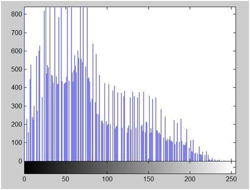
In this case the contrast of the image can be calculated as
Contrast = 240
Hence we can say that the contrast of the image is increased.
Note: this method of increasing contrast doesnot work always, but it fails on some cases.
Failing of histogram stretching
As we have discussed , that the algorithm fails on some cases. Those cases include images with when there is pixel intensity 0 and 255 are present in the image
Because when pixel intensities 0 and 255 are present in an image , then in that case they become the minimum and maximum pixel intensity which ruins the formula like this.
Original Formula
Putting fail case values in the formula:
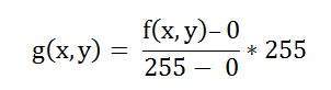
Simplify that expression gives
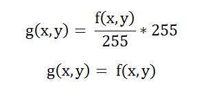
That means the output image is equal to the processed image. That means there is no effect of histogram stretching has been done at this image.
Introduction to Probability
PMF and CDF both terms belongs to probability and statistics. Now the question that should arise in your mind , is that why are we studying probability. It is because these two concepts of PMF and CDF are going to be used in the next tutorial of Histogram equalization. So if you dont know how to calculate PMF and CDF , you can not apply histogram equalization on your image
.What is PMF?
PMF stands for probability mass function. As it name suggest , it gives the probability of each number in the data set or you can say that it basically gives the count or frequency of each element.
How PMF is calculated:
We will calculate PMF from two different ways. First from a matrix , because in the next tutorial , we have to calculate the PMF from a matrix , and an image is nothing more then a two dimensional matrix.
Then we will take another example in which we will calculate PMF from the histogram.
Consider this matrix.
| 1 | 2 | 7 | 5 | 6 |
| 7 | 2 | 3 | 4 | 5 |
| 0 | 1 | 5 | 7 | 3 |
| 1 | 2 | 5 | 6 | 7 |
| 6 | 1 | 0 | 3 | 4 |
Now if we were to calculate the PMF of this matrix , here how we are going to do it.
At first , we will take the first value in the matrix , and then we will count , how much time this value appears in the whole matrix. After count they can either be represented in a histogram , or in a table like this below.
PMF
| 0 | 2 | 2/25 |
| 1 | 4 | 4/25 |
| 2 | 3 | 3/25 |
| 3 | 3 | 3/25 |
| 4 | 2 | 2/25 |
| 5 | 4 | 4/25 |
| 6 | 3 | 3/25 |
| 7 | 4 | 4/25 |
Note that the sum of the count must be equal to total number of values.
Calculating PMF from histogram
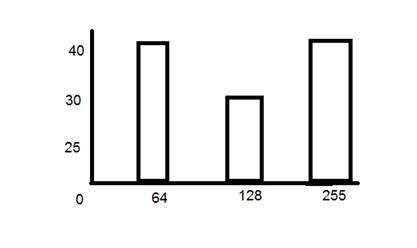
The above histogram shows frequency of gray level values for an 8 bits per pixel image.
Now if we have to calculate its PMF , we will simple look at the count of each bar from vertical axis and then divide it by total count.
So the PMF of the above histogram is this.
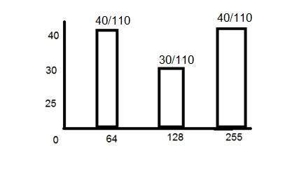
Another important thing to note in the above histogram is that it is not monotonically increasing. So in order to increase it monotonically, we will calculate its CDF.
What is CDF?
CDF stands for cumulative distributive function. It is a function that calculates the cumulative sum of all the values that are calculated by PMF. It basically sums the previous one.
How it is calculated?
We will calculate CDF using a histogram. Here how it is done. Consider the histogram shown above which shows PMF.
Since this histogram is not increasing monotonically , so will make it grow monotonically.
We will simply keep the first value as it is , and then in the 2nd value , we will add the first one and so on.
Here is the CDF of the above PMF function.
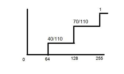
Now as you can see from the graph above , that the first value of PMF remain as it is. The second value of PMF is added in the first value and placed over 128. The third value of PMF is added in the second value of CDF , that gives 110/110 which is equal to 1.
And also now , the function is growing monotonically which is necessary condition for histogram equalization.
PMF and CDF usage in histogram equalization
Histogram equalization.
Histogram equalization is discussed in the next tutorial but a brief introduction of histogram equalization is given below.
Histogram equalization is used for enhancing the contrast of the images.
PMF and CDF are both use in histogram equalization as it is described in the beginning of this tutorial. In the histogram equalization , the first and the second step are PMF and CDF. Since in histogram equalization , we have to equalize all the pixel values of an image. So PMF helps us calculating the probability of each pixel value in an image. And CDF gives us the cumulative sum of these values. Further on , this CDF is multiplied by levels , to find the new pixel intensities , which are mapped into old values , and your histogram is equalized.
Histogram Equalization
We have already seen that contrast can be increased using histogram stretching. In this tutorial we will see that how histogram equalization can be used to enhance contrast.
Before performing histogram equalization, you must know two important concepts used in equalizing histograms. These two concepts are known as PMF and CDF.
They are discussed in our tutorial of PMF and CDF. Please visit them in order to successfully grasp the concept of histogram equalization.
Histogram Equalization:
Histogram equalization is used to enhance contrast. It is not necessary that contrast will always be increase in this. There may be some cases were histogram equalization can be worse. In that cases the contrast is decreased.
Lets start histogram equalization by taking this image below as a simple image.
Image
Histogram of this image:
The histogram of this image has been shown below.
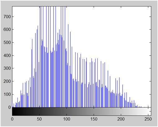
Now we will perform histogram equalization to it.
PMF:
First we have to calculate the PMF (probability mass function) of all the pixels in this image. If you donot know how to calculate PMF, please visit our tutorial of PMF calculation.
CDF:
Our next step involves calculation of CDF (cumulative distributive function). Again if you donot know how to calculate CDF , please visit our tutorial of CDF calculation.
Calculate CDF according to gray levels
Lets for instance consider this , that the CDF calculated in the second step looks like this.
| Gray Level Value | CDF |
|---|---|
| 0 | 0.11 |
| 1 | 0.22 |
| 2 | 0.55 |
| 3 | 0.66 |
| 4 | 0.77 |
| 5 | 0.88 |
| 6 | 0.99 |
| 7 | 1 |
Then in this step you will multiply the CDF value with (Gray levels (minus) 1) .
Considering we have an 3 bpp image. Then number of levels we have are 8. And 1 subtracts 8 is 7. So we multiply CDF by 7. Here what we got after multiplying.
| Gray Level Value | CDF | CDF * (Levels-1) |
|---|---|---|
| 0 | 0.11 | 0 |
| 1 | 0.22 | 1 |
| 2 | 0.55 | 3 |
| 3 | 0.66 | 4 |
| 4 | 0.77 | 5 |
| 5 | 0.88 | 6 |
| 6 | 0.99 | 6 |
| 7 | 1 | 7 |
Now we have is the last step , in which we have to map the new gray level values into number of pixels.
Lets assume our old gray levels values has these number of pixels.
| Gray Level Value | Frequency |
|---|---|
| 0 | 2 |
| 1 | 4 |
| 2 | 6 |
| 3 | 8 |
| 4 | 10 |
| 5 | 12 |
| 6 | 14 |
| 7 | 16 |
Now if we map our new values to , then this is what we got.
| Gray Level Value | New Gray Level Value | Frequency |
|---|---|---|
| 0 | 0 | 2 |
| 1 | 1 | 4 |
| 2 | 3 | 6 |
| 3 | 4 | 8 |
| 4 | 5 | 10 |
| 5 | 6 | 12 |
| 6 | 6 | 14 |
| 7 | 7 | 16 |
Now map these new values you are onto histogram , and you are done.
Lets apply this technique to our original image. After applying we got the following image and its following histogram.
Histogram Equalization Image
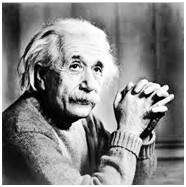
Cumulative Distributive function of this image
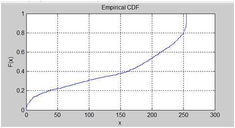
Histogram Equalization histogram
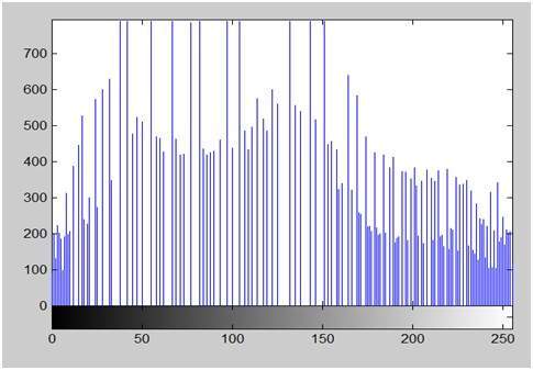
Comparing both the histograms and images
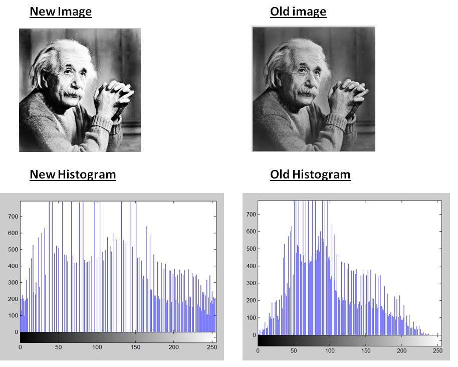
Conclusion
As you can clearly see from the images that the new image contrast has been enhanced and its histogram has also been equalized. There is also one important thing to be note here that during histogram equalization the overall shape of the histogram changes, where as in histogram stretching the overall shape of histogram remains same.
Gray Level Transformation
We have discussed some of the basic transformations in our tutorial of Basic transformation. In this tutorial we will look at some of the basic gray level transformations.
Image enhancement
Enhancing an image provides better contrast and a more detailed image as compare to non enhanced image. Image enhancement has very applications. It is used to enhance medical images , images captured in remote sensing , images from satellite e.t.c
The transformation function has been given below
s = T ( r )
where r is the pixels of the input image and s is the pixels of the output image. T is a transformation function that maps each value of r to each value of s. Image enhancement can be done through gray level transformations which are discussed below.
Gray level transformation
There are three basic gray level transformation.
Linear
Logarithmic
Power – law
The overall graph of these transitions has been shown below.
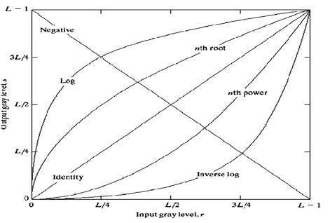
Linear transformation
First we will look at the linear transformation. Linear transformation includes simple identity and negative transformation. Identity transformation has been discussed in our tutorial of image transformation, but a brief description of this transformation has been given here.
Identity transition is shown by a straight line. In this transition, each value of the input image is directly mapped to each other value of output image. That results in the same input image and output image. And hence is called identity transformation. It has been shown below
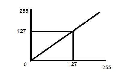
Negative transformation
The second linear transformation is negative transformation, which is invert of identity transformation. In negative transformation, each value of the input image is subtracted from the L-1 and mapped onto the output image.
The result is somewhat like this.
Input Image

Output Image
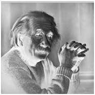
In this case the following transition has been done.
s = (L – 1) – r
since the input image of Einstein is an 8 bpp image , so the number of levels in this image are 256. Putting 256 in the equation, we get this
s = 255 – r
So each value is subtracted by 255 and the result image has been shown above. So what happens is that , the lighter pixels become dark and the darker picture becomes light. And it results in image negative.
It has been shown in the graph below.
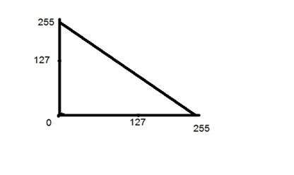
Logarithmic transformations:
Logarithmic transformation further contains two type of transformation. Log transformation and inverse log transformation.
Log transformation
The log transformations can be defined by this formula
s = c log(r + 1).
Where s and r are the pixel values of the output and the input image and c is a constant. The value 1 is added to each of the pixel value of the input image because if there is a pixel intensity of 0 in the image, then log (0) is equal to infinity. So 1 is added , to make the minimum value at least 1.
During log transformation , the dark pixels in an image are expanded as compare to the higher pixel values. The higher pixel values are kind of compressed in log transformation. This result in following image enhancement.
The value of c in the log transform adjust the kind of enhancement you are looking for.
Input Image
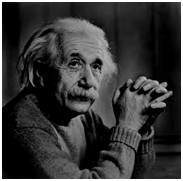
Log Tranform Image
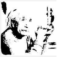
The inverse log transform is opposite to log transform.
Power – Law transformations
There are further two transformation is power law transformations, that include nth power and nth root transformation. These transformations can be given by the expression:
s=cr^γ
This symbol γ is called gamma, due to which this transformation is also known as gamma transformation.
Variation in the value of γ varies the enhancement of the images. Different display devices / monitors have their own gamma correction, that’s why they display their image at different intensity.
This type of transformation is used for enhancing images for different type of display devices. The gamma of different display devices is different. For example Gamma of CRT lies in between of 1.8 to 2.5 , that means the image displayed on CRT is dark.
Correcting gamma.
s=cr^γ
s=cr^(1/2.5)
The same image but with different gamma values has been shown here.
For example:
Gamma = 10
Gamma = 8
Gamma = 6
Concept of Convolution
This tutorial is about one of the very important concept of signals and system. We will completely discuss convolution. What is it? Why is it? What can we achieve with it?
We will start discussing convolution from the basics of image processing.
What is image processing.
As we have discussed in the introduction to image processing tutorials and in the signal and system that image processing is more or less the study of signals and systems because an image is nothing but a two dimensional signal.
Also we have discussed , that in image processing , we are developing a system whose input is an image and output would be an image. This is pictorially represented as.
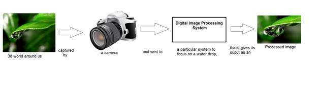
The box is that is shown in the above figure labeled as “Digital Image Processing system” could be thought of as a black box
It can be better represented as:
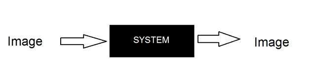
Where have we reached until now
Till now we have discussed two important methods to manipulate images. Or in other words we can say that, our black box works in two different ways till now.
The two different ways of manipulating images were
Graphs (Histograms)
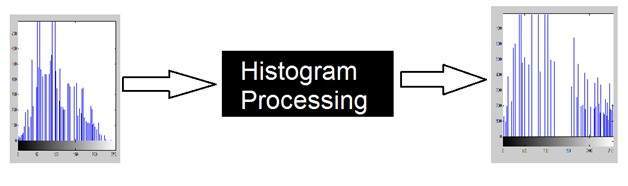
This method is known as histogram processing. We have discussed it in detail in previous tutorials for increase contrast , image enhancement , brightness e.t.c
Transformation functions
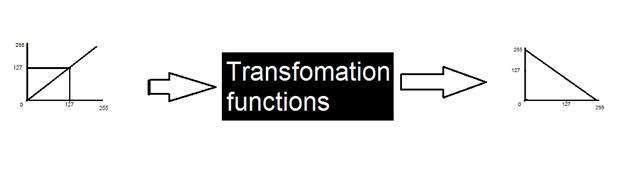
This method is known as transformations , in which we discussed different type of transformations and some gray level transformations
Another way of dealing images
Here we are going to discuss another method of dealing with images. This other method is known as convolution. Usually the black box(system) used for image processing is an LTI system or linear time invariant system. By linear we mean that such a system where output is always linear , neither log nor exponent or any other. And by time invariant we means that a system which remains same during time.
So now we are going to use this third method. It can be represented as.
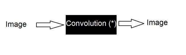
It can be mathematically represented as two ways
g(x,y) = h(x,y) * f(x,y)
It can be explained as the “mask convolved with an image”.
Or
g(x,y) = f(x,y) * h(x,y)
It can be explained as “image convolved with mask”.
There are two ways to represent this because the convolution operator(*) is commutative. The h(x,y) is the mask or filter.
What is mask?
Mask is also a signal. It can be represented by a two dimensional matrix. The mask is usually of the order of 1x1, 3x3, 5x5 , 7x7 . A mask should always be in odd number , because other wise you cannot find the mid of the mask. Why do we need to find the mid of the mask. The answer lies below, in topic of , how to perform convolution?
How to perform convolution?
In order to perform convolution on an image , following steps should be taken.
Flip the mask (horizontally and vertically) only once
Slide the mask onto the image.
Multiply the corresponding elements and then add them
Repeat this procedure until all values of the image has been calculated.
Example of convolution
Let’s perform some convolution. Step 1 is to flip the mask.
Mask:
Let’s take our mask to be this.
| 1 | 2 | 3 |
| 4 | 5 | 6 |
| 7 | 8 | 9 |
Flipping the mask horizontally
| 3 | 2 | 1 |
| 6 | 5 | 4 |
| 9 | 8 | 7 |
Flipping the mask vertically
| 9 | 8 | 7 |
| 6 | 5 | 4 |
| 3 | 2 | 1 |
Image:
Let’s consider an image to be like this
| 2 | 4 | 6 |
| 8 | 10 | 12 |
| 14 | 16 | 18 |
Convolution
Convolving mask over image. It is done in this way. Place the center of the mask at each element of an image. Multiply the corresponding elements and then add them , and paste the result onto the element of the image on which you place the center of mask.
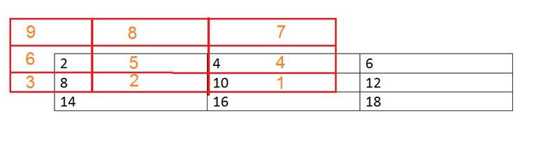
The box in red color is the mask , and the values in the orange are the values of the mask. The black color box and values belong to the image. Now for the first pixel of the image , the value will be calculated as
First pixel = (5*2) + (4*4) + (2*8) + (1*10)
= 10 + 16 + 16 + 10
= 52
Place 52 in the original image at the first index and repeat this procedure for each pixel of the image.
Why Convolution
Convolution can achieve something, that the previous two methods of manipulating images can’t achieve. Those include the blurring , sharpening , edge detection , noise reduction e.t.c
Concept of Mask
What is a mask.
A mask is a filter. Concept of masking is also known as spatial filtering. Masking is also known as filtering. In this concept we just deal with the filtering operation that is performed directly on the image.
A sample mask has been shown below
| -1 | 0 | 1 |
| -1 | 0 | 1 |
| -1 | 0 | 1 |
What is filtering.
The process of filtering is also known as convolving a mask with an image. As this process is same of convolution so filter masks are also known as convolution masks.
How it is done.
The general process of filtering and applying masks is consists of moving the filter mask from point to point in an image. At each point (x,y) of the original image, the response of a filter is calculated by a pre defined relationship. All the filters values are pre defined and are a standard.
Types of filters
Generally there are two types of filters. One is called as linear filters or smoothing filters and others are called as frequency domain filters.
Why filters are used?
Filters are applied on image for multiple purposes. The two most common uses are as following:
Filters are used for Blurring and noise reduction
Filters are used or edge detection and sharpness
Blurring and noise reduction:
Filters are most commonly used for blurring and for noise reduction. Blurring is used in pre processing steps, such as removal of small details from an image prior to large object extraction.
Masks for blurring.
The common masks for blurring are.
Box filter
Weighted average filter
In the process of blurring we reduce the edge content in an image and try to make the transitions between different pixel intensities as smooth as possible.
Noise reduction is also possible with the help of blurring.
Edge Detection and sharpness:
Masks or filters can also be used for edge detection in an image and to increase sharpness of an image.
What are edges.
We can also say that sudden changes of discontinuities in an image are called as edges. Significant transitions in an image are called as edges.A picture with edges is shown below.
Original picture.

Same picture with edges
Concept of Blurring
A brief introduction of blurring has been discussed in our previous tutorial of concept of masks, but we are formally going to discuss it here.
Blurring
In blurring , we simple blur an image. An image looks more sharp or more detailed if we are able to perceive all the objects and their shapes correctly in it. For example. An image with a face, looks clear when we are able to identify eyes , ears , nose , lips , forehead e.t.c very clear. This shape of an object is due to its edges. So in blurring , we simple reduce the edge content and makes the transition form one color to the other very smooth.
Blurring vs zooming.
You might have seen a blurred image when you zoom an image. When you zoom an image using pixel replication , and zooming factor is increased, you saw a blurred image. This image also has less details , but it is not true blurring.
Because in zooming , you add new pixels to an image , that increase the overall number of pixels in an image , whereas in blurring , the number of pixels of a normal image and a blurred image remains the same.
Common example of a blurred image.
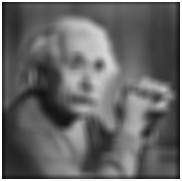
Types of filters.
Blurring can be achieved by many ways. The common type of filters that are used to perform blurring are.
Mean filter
Weighted average filter
Gaussian filter
Out of these three , we are going to discuss the first two here and Gaussian will be discussed later on in the upcoming tutorials.
Mean filter.
Mean filter is also known as Box filter and average filter. A mean filter has the following properties.
It must be odd ordered
The sum of all the elements should be 1
All the elements should be same
If we follow this rule , then for a mask of 3x3. We get the following result.
| 1/9 | 1/9 | 1/9 |
| 1/9 | 1/9 | 1/9 |
| 1/9 | 1/9 | 1/9 |
Since it is a 3x3 mask, that means it has 9 cells. The condition that all the element sum should be equal to 1 can be achieved by dividing each value by 9. As
1/9 + 1/9 + 1/9 + 1/9 + 1/9 + 1/9 + 1/9 + 1/9 + 1/9 = 9/9 = 1
The result of a mask of 3x3 on an image is shown below.
Original Image:

Blurred Image
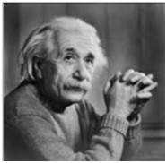
May be the results are not much clear. Let’s increase the blurring. The blurring can be increased by increasing the size of the mask. The more is the size of the mask , the more is the blurring. Because with greater mask , greater number of pixels are catered and one smooth transition is defined.
The result of a mask of 5x5 on an image is shown below.
Original Image:

Blurred Image:
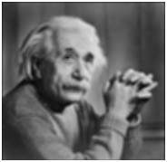
Same way if we increase the mask , the blurring would be more and the results are shown below.
The result of a mask of 7x7 on an image is shown below.
Original Image:

Blurred Image:

The result of a mask of 9x9 on an image is shown below.
Original Image:

Blurred Image:
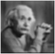
The result of a mask of 11x11 on an image is shown below.
Original Image:

Blurred Image:
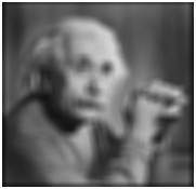
Weighted average filter.
In weighted average filter, we gave more weight to the center value. Due to which the contribution of center becomes more then the rest of the values. Due to weighted average filtering , we can actually control the blurring.
Properties of the weighted average filter are.
It must be odd ordered
The sum of all the elements should be 1
The weight of center element should be more then all of the other elements
Filter 1
| 1 | 1 | 1 |
| 1 | 2 | 1 |
| 1 | 1 | 1 |
The two properties are satisfied which are (1 and 3). But the property 2 is not satisfied. So in order to satisfy that we will simple divide the whole filter by 10, or multiply it with 1/10.
Filter 2
| 1 | 1 | 1 |
| 1 | 10 | 1 |
| 1 | 1 | 1 |
Dividing factor = 18.
Concept of Edge Detection
We have discussed briefly about edge detection in our tutorial of introduction to masks. We will formally discuss edge detection here.
What are edges.
We can also say that sudden changes of discontinuities in an image are called as edges. Significant transitions in an image are called as edges.
Types of edges.
Geenerally edges are of three types:
Horizontal edges
Vertical Edges
Diagonal Edges
Why detect edges.
Most of the shape information of an image is enclosed in edges. So first we detect these edges in an image and by using these filters and then by enhancing those areas of image which contains edges, sharpness of the image will increase and image will become clearer.
Here are some of the masks for edge detection that we will discuss in the upcoming tutorials.
Prewitt Operator
Sobel Operator
Robinson Compass Masks
Krisch Compass Masks
Laplacian Operator.
Above mentioned all the filters are Linear filters or smoothing filters.
Prewitt Operator
Prewitt operator is used for detecting edges horizontally and vertically.
Sobel Operator
The sobel operator is very similar to Prewitt operator. It is also a derivate mask and is used for edge detection. It also calculates edges in both horizontal and vertical direction.
Robinson Compass Masks
This operator is also known as direction mask. In this operator we take one mask and rotate it in all the 8 compass major directions to calculate edges of each direction.
Kirsch Compass Masks
Kirsch Compass Mask is also a derivative mask which is used for finding edges. Kirsch mask is also used for calculating edges in all the directions.
Laplacian Operator.
Laplacian Operator is also a derivative operator which is used to find edges in an image. Laplacian is a second order derivative mask. It can be further divided into positive laplacian and negative laplacian.
All these masks find edges. Some find horizontally and vertically, some find in one direction only and some find in all the directions. The next concept that comes after this is sharpening which can be done once the edges are extracted from the image
Sharpening :
Sharpening is opposite to the blurring. In blurring, we reduce the edge content and in sharpneng , we increase the edge content. So in order to increase the edge content in an image , we have to find edges first.
Edges can be find by one of the any method described above by using any operator. After finding edges , we will add those edges on an image and thus the image would have more edges , and it would look sharpen.
This is one way of sharpening an image.
The sharpen image is shown below.
Original Image

Sharpen Image

Prewitt Operator
Prewitt operator is used for edge detection in an image. It detects two types of edges:
Horizontal edges
Vertical Edges
Edges are calculated by using difference between corresponding pixel intensities of an image. All the masks that are used for edge detection are also known as derivative masks. Because as we have stated many times before in this series of tutorials that image is also a signal so changes in a signal can only be calculated using differentiation. So that’s why these operators are also called as derivative operators or derivative masks.
All the derivative masks should have the following properties:
Opposite sign should be present in the mask.
Sum of mask should be equal to zero.
More weight means more edge detection.
Prewitt operator provides us two masks one for detecting edges in horizontal direction and another for detecting edges in an vertical direction.
Vertical direction:
| -1 | 0 | 1 |
| -1 | 0 | 1 |
| -1 | 0 | 1 |
Above mask will find the edges in vertical direction and it is because the zeros column in the vertical direction. When you will convolve this mask on an image, it will give you the vertical edges in an image.
How it works:
When we apply this mask on the image it prominent vertical edges. It simply works like as first order derivate and calculates the difference of pixel intensities in a edge region. As the center column is of zero so it does not include the original values of an image but rather it calculates the difference of right and left pixel values around that edge. This increase the edge intensity and it become enhanced comparatively to the original image.
Horizontal Direction:
| -1 | -1 | -1 |
| 0 | 0 | 0 |
| 1 | 1 | 1 |
Above mask will find edges in horizontal direction and it is because that zeros column is in horizontal direction. When you will convolve this mask onto an image it would prominent horizontal edges in the image.
How it works:
This mask will prominent the horizontal edges in an image. It also works on the principle of above mask and calculates difference among the pixel intensities of a particular edge. As the center row of mask is consist of zeros so it does not include the original values of edge in the image but rather it calculate the difference of above and below pixel intensities of the particular edge. Thus increasing the sudden change of intensities and making the edge more visible. Both the above masks follow the principle of derivate mask. Both masks have opposite sign in them and both masks sum equals to zero. The third condition will not be applicable in this operator as both the above masks are standardize and we can’t change the value in them.
Now it’s time to see these masks in action:
Sample Image:
Following is a sample picture on which we will apply above two masks one at time.

After applying Vertical Mask:
After applying vertical mask on the above sample image, following image will be obtained. This image contains vertical edges. You can judge it more correctly by comparing with horizontal edges picture.
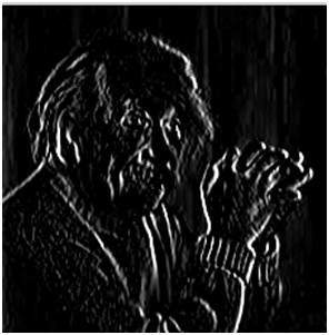
After applying Horizontal Mask:
After applying horizontal mask on the above sample image, following image will be obtained.
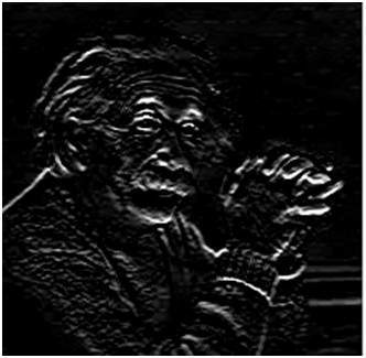
Comparison:
As you can see that in the first picture on which we apply vertical mask, all the vertical edges are more visible than the original image. Similarly in the second picture we have applied the horizontal mask and in result all the horizontal edges are visible. So in this way you can see that we can detect both horizontal and vertical edges from an image.
Sobel Operator
The sobel operator is very similar to Prewitt operator. It is also a derivate mask and is used for edge detection. Like Prewitt operator sobel operator is also used to detect two kinds of edges in an image:
Vertical direction
Horizontal direction
Difference with Prewitt Operator:
The major difference is that in sobel operator the coefficients of masks are not fixed and they can be adjusted according to our requirement unless they do not violate any property of derivative masks.
Following is the vertical Mask of Sobel Operator:
| -1 | 0 | 1 |
| -2 | 0 | 2 |
| -1 | 0 | 1 |
This mask works exactly same as the Prewitt operator vertical mask. There is only one difference that is it has “2” and “-2” values in center of first and third column. When applied on an image this mask will highlight the vertical edges.
How it works:
When we apply this mask on the image it prominent vertical edges. It simply works like as first order derivate and calculates the difference of pixel intensities in a edge region.
As the center column is of zero so it does not include the original values of an image but rather it calculates the difference of right and left pixel values around that edge. Also the center values of both the first and third column is 2 and -2 respectively.
This give more weight age to the pixel values around the edge region. This increase the edge intensity and it become enhanced comparatively to the original image.
Following is the horizontal Mask of Sobel Operator:
| -1 | -2 | -1 |
| 0 | 0 | 0 |
| 1 | 2 | 1 |
Above mask will find edges in horizontal direction and it is because that zeros column is in horizontal direction. When you will convolve this mask onto an image it would prominent horizontal edges in the image. The only difference between it is that it have 2 and -2 as a center element of first and third row.
How it works:
This mask will prominent the horizontal edges in an image. It also works on the principle of above mask and calculates difference among the pixel intensities of a particular edge. As the center row of mask is consist of zeros so it does not include the original values of edge in the image but rather it calculate the difference of above and below pixel intensities of the particular edge. Thus increasing the sudden change of intensities and making the edge more visible.
Now it’s time to see these masks in action:
Sample Image:
Following is a sample picture on which we will apply above two masks one at time.

After applying Vertical Mask:
After applying vertical mask on the above sample image, following image will be obtained.
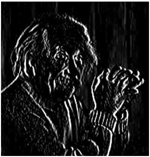
After applying Horizontal Mask:
After applying horizontal mask on the above sample image, following image will be obtained
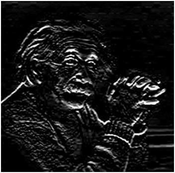
Comparison:
As you can see that in the first picture on which we apply vertical mask, all the vertical edges are more visible than the original image. Similarly in the second picture we have applied the horizontal mask and in result all the horizontal edges are visible.
So in this way you can see that we can detect both horizontal and vertical edges from an image. Also if you compare the result of sobel operator with Prewitt operator, you will find that sobel operator finds more edges or make edges more visible as compared to Prewitt Operator.
This is because in sobel operator we have allotted more weight to the pixel intensities around the edges.
Applying more weight to mask
Now we can also see that if we apply more weight to the mask, the more edges it will get for us. Also as mentioned in the start of the tutorial that there is no fixed coefficients in sobel operator, so here is another weighted operator
| -1 | 0 | 1 |
| -5 | 0 | 5 |
| -1 | 0 | 1 |
If you can compare the result of this mask with of the Prewitt vertical mask, it is clear that this mask will give out more edges as compared to Prewitt one just because we have allotted more weight in the mask.
Robinson Compass Mask
Robinson compass masks are another type of derrivate mask which is used for edge detection. This operator is also known as direction mask. In this operator we take one mask and rotate it in all the 8 compass major directions that are following:
North
North West
West
South West
South
South East
East
North East
There is no fixed mask. You can take any mask and you have to rotate it to find edges in all the above mentioned directions. All the masks are rotated on the bases of direction of zero columns.
For example let’s see the following mask which is in North Direction and then rotate it to make all the direction masks.
North Direction Mask
| -1 | 0 | 1 |
| -2 | 0 | 2 |
| -1 | 0 | 1 |
North West Direction Mask
| 0 | 1 | 2 |
| -1 | 0 | 1 |
| -2 | -1 | 0 |
West Direction Mask
| 1 | 2 | 1 |
| 0 | 0 | 0 |
| -1 | -2 | -1 |
South West Direction Mask
| 2 | 1 | 0 |
| 1 | 0 | -1 |
| 0 | -1 | -2 |
South Direction Mask
| 1 | 0 | -1 |
| 2 | 0 | -2 |
| 1 | 0 | -1 |
South East Direction Mask
| 0 | -1 | -2 |
| 1 | 0 | -1 |
| 2 | 1 | 0 |
East Direction Mask
| -1 | -2 | -1 |
| 0 | 0 | 0 |
| 1 | 2 | 1 |
North East Direction Mask
| -2 | -1 | 0 |
| -1 | 0 | 1 |
| 0 | 1 | 2 |
As you can see that all the directions are covered on the basis of zeros direction. Each mask will give you the edges on its direction. Now let’s see the result of the entire above masks. Suppose we have a sample picture from which we have to find all the edges. Here is our sample picture:
Sample Picture:

Now we will apply all the above filters on this image and we get the following result.
North Direction Edges
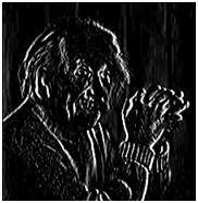
North West Direction Edges
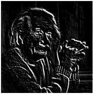
West Direction Edges
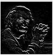
South West Direction Edges
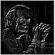
South Direction Edges
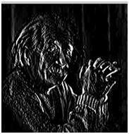
South East Direction Edges
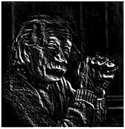
East Direction Edges
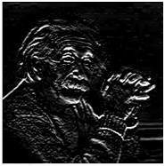
North East Direction Edges
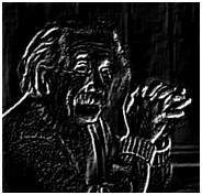
As you can see that by applying all the above masks you will get edges in all the direction. Result is also depends on the image. Suppose there is an image, which do not have any North East direction edges so then that mask will be ineffective.
Krisch Compass Mask
Kirsch Compass Mask is also a derivative mask which is used for finding edges. This is also like Robinson compass find edges in all the eight directions of a compass. The only difference between Robinson and kirsch compass masks is that in Kirsch we have a standard mask but in Kirsch we change the mask according to our own requirements.
With the help of Kirsch Compass Masks we can find edges in the following eight directions.
North
North West
West
South West
South
South East
East
North East
We take a standard mask which follows all the properties of a derivative mask and then rotate it to find the edges.
For example let’s see the following mask which is in North Direction and then rotate it to make all the direction masks.
North Direction Mask
| -3 | -3 | 5 |
| -3 | 0 | 5 |
| -3 | -3 | 5 |
North West Direction Mask
| -3 | 5 | 5 |
| -3 | 0 | 5 |
| -3 | -3 | -3 |
West Direction Mask
| 5 | 5 | 5 |
| -3 | 0 | -3 |
| -3 | -3 | -3 |
South West Direction Mask
| 5 | 5 | -3 |
| 5 | 0 | -3 |
| -3 | -3 | -3 |
South Direction Mask
| 5 | -3 | -3 |
| 5 | 0 | -3 |
| 5 | -3 | -3 |
South East Direction Mask
| -3 | -3 | -3 |
| 5 | 0 | -3 |
| 5 | 5 | -3 |
East Direction Mask
| -3 | -3 | -3 |
| -3 | 0 | -3 |
| 5 | 5 | 5 |
North East Direction Mask
| -3 | -3 | -3 |
| -3 | 0 | 5 |
| -3 | 5 | 5 |
As you can see that all the directions are covered and each mask will give you the edges of its own direction. Now to help you better understand the concept of these masks we will apply it on a real image. Suppose we have a sample picture from which we have to find all the edges. Here is our sample picture:
Sample Picture
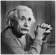
Now we will apply all the above filters on this image and we get the following result.
North Direction Edges
North West Direction Edges
West Direction Edges
South West Direction Edges
South Direction Edges
South East Direction Edges
East Direction Edges
North East Direction Edges
As you can see that by applying all the above masks you will get edges in all the direction. Result is also depends on the image. Suppose there is an image, which do not have any North East direction edges so then that mask will be ineffective.
Laplacian Operator
Laplacian Operator is also a derivative operator which is used to find edges in an image. The major difference between Laplacian and other operators like Prewitt, Sobel, Robinson and Kirsch is that these all are first order derivative masks but Laplacian is a second order derivative mask. In this mask we have two further classifications one is Positive Laplacian Operator and other is Negative Laplacian Operator.
Another difference between Laplacian and other operators is that unlike other operators Laplacian didn’t take out edges in any particular direction but it take out edges in following classification.
Inward Edges
Outward Edges
Let’s see that how Laplacian operator works.
Positive Laplacian Operator:
In Positive Laplacian we have standard mask in which center element of the mask should be negative and corner elements of mask should be zero.
| 0 | 1 | 0 |
| 1 | -4 | 1 |
| 0 | 1 | 0 |
Positive Laplacian Operator is use to take out outward edges in an image.
Negative Laplacian Operator:
In negative Laplacian operator we also have a standard mask, in which center element should be positive. All the elements in the corner should be zero and rest of all the elements in the mask should be -1.
| 0 | -1 | 0 |
| -1 | 4 | -1 |
| 0 | -1 | 0 |
Negative Laplacian operator is use to take out inward edges in an image
How it works:
Laplacian is a derivative operator; its uses highlight gray level discontinuities in an image and try to deemphasize regions with slowly varying gray levels. This operation in result produces such images which have grayish edge lines and other discontinuities on a dark background. This produces inward and outward edges in an image
The important thing is how to apply these filters onto image. Remember we can’t apply both the positive and negative Laplacian operator on the same image. we have to apply just one but the thing to remember is that if we apply positive Laplacian operator on the image then we subtract the resultant image from the original image to get the sharpened image. Similarly if we apply negative Laplacian operator then we have to add the resultant image onto original image to get the sharpened image.
Let’s apply these filters onto an image and see how it will get us inward and outward edges from an image. Suppose we have a following sample image.
Sample Image

After applying Positive Laplacian Operator:
After applying positive Laplacian operator we will get the following image.
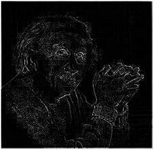
After applying Negative Laplacian Operator:
After applying negative Laplacian operator we will get the following image.
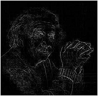
Introduction to Frequency domain
We have deal with images in many domains. Now we are processing signals (images) in frequency domain. Since this Fourier series and frequency domain is purely mathematics , so we will try to minimize that math’s part and focus more on its use in DIP.
Frequency domain analysis
Till now , all the domains in which we have analyzed a signal , we analyze it with respect to time. But in frequency domain we don’t analyze signal with respect to time , but with respect of frequency.
Difference between spatial domain and frequency domain.
In spatial domain , we deal with images as it is. The value of the pixels of the image change with respect to scene. Whereas in frequency domain , we deal with the rate at which the pixel values are changing in spatial domain.
For simplicity , Let’s put it this way.
Spatial domain
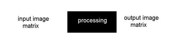
In simple spatial domain , we directly deal with the image matrix. Whereas in frequency domain , we deal an image like this.
Frequency Domain
We first transform the image to its frequency distribution. Then our black box system perform what ever processing it has to performed , and the output of the black box in this case is not an image , but a transformation. After performing inverse transformation , it is converted into an image which is then viewed in spatial domain.
It can be pictorially viewed as
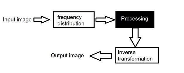
Here we have used the word transformation. What does it actually mean?
Transformation.
A signal can be converted from time domain into frequency domain using mathematical operators called transforms. There are many kind of transformation that does this. Some of them are given below.
Fourier Series
Fourier transformation
Laplace transform
Z transform
Out of all these , we will thoroughly discuss Fourier series and Fourier transformation in our next tutorial.
Frequency components
Any image in spatial domain can be represented in a frequency domain. But what do this frequencies actually mean.
We will divide frequency components into two major components.
High frequency components
High frequency components correspond to edges in an image.
Low frequency components
Low frequency components in an image correspond to smooth regions.
Fourier Series and Transform
In the last tutorial of Frequency domain analysis, we discussed that Fourier series and Fourier transform are used to convert a signal to frequency domain.
Fourier
Fourier was a mathematician in 1822. He give Fourier series and Fourier transform to convert a signal into frequency domain.
Fourier Series
Fourier series simply states that , periodic signals can be represented into sum of sines and cosines when multiplied with a certain weight.It further states that periodic signals can be broken down into further signals with the following properties.
The signals are sines and cosines
The signals are harmonics of each other
It can be pictorially viewed as

In the above signal , the last signal is actually the sum of all the above signals. This was the idea of the Fourier.
How it is calculated.
Since as we have seen in the frequency domain , that in order to process an image in frequency domain , we need to first convert it using into frequency domain and we have to take inverse of the output to convert it back into spatial domain. That’s why both Fourier series and Fourier transform has two formulas. One for conversion and one converting it back to the spatial domain.
Fourier series
The Fourier series can be denoted by this formula.
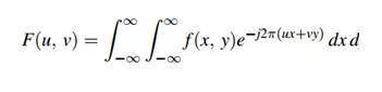
The inverse can be calculated by this formula.
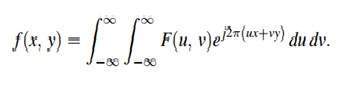
Fourier transform
The Fourier transform simply states that that the non periodic signals whose area under the curve is finite can also be represented into integrals of the sines and cosines after being multiplied by a certain weight.
The Fourier transform has many wide applications that include , image compression (e.g JPEG compression) , filtrering and image analysis.
Difference between Fourier series and transform
Although both Fourier series and Fourier transform are given by Fourier , but the difference between them is Fourier series is applied on periodic signals and Fourier transform is applied for non periodic signals
Which one is applied on images.
Now the question is that which one is applied on the images , the Fourier series or the Fourier transform. Well , the answer to this question lies in the fact that what images are. Images are non – periodic. And since the images are non periodic , so Fourier transform is used to convert them into frequency domain.
Discrete fourier transform.
Since we are dealing with images, and infact digital images , so for digital images we will be working on discrete fourier transform
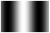
Consider the above Fourier term of a sinusoid. It include three things.
Spatial Frequency
Magnitude
Phase
The spatial frequency directly relates with the brightness of the image. The magnitude of the sinusoid directly relates with the contrast. Contrast is the difference between maximum and minimum pixel intensity. Phase contains the color information.
The formula for 2 dimensional discrete Fourier transform is given below.
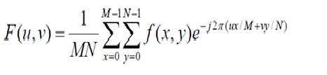
The discrete Fourier transform is actually the sampled Fourier transform, so it contains some samples that denotes an image. In the above formula f(x,y) denotes the image , and F(u,v) denotes the discrete Fourier transform. The formula for 2 dimensional inverse discrete Fourier transform is given below.
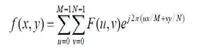
The inverse discrete Fourier transform converts the Fourier transform back to the image
Consider this signal.
Now we will see an image , whose we will calculate FFT magnitude spectrum and then shifted FFT magnitude spectrum and then we will take Log of that shifted spectrum.
Original Image
The Fourier transform magnitude spectrum
The Shifted Fourier transform
The Shifted Magnitude Spectrum
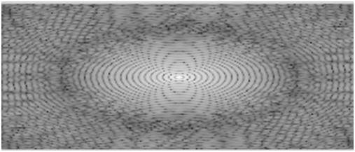
Convolution Theorem
In the last tutorial , we discussed about the images in frequency domain. In this tutorial , we are going to define a relationship between frequency domain and the images(spatial domain).
For example:
Consider this example.

The same image in the frequency domain can be represented as.
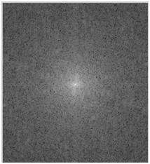
Now what’s the relationship between image or spatial domain and frequency domain. This relationship can be explained by a theorem which is called as Convolution theorem.
Convolution Theorem
The relationship between the spatial domain and the frequency domain can be established by convolution theorem.
The convolution theorem can be represented as.
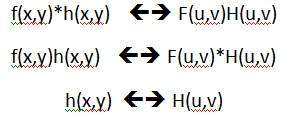
It can be stated as the convolution in spatial domain is equal to filtering in frequency domain and vice versa.
The filtering in frequency domain can be represented as following:
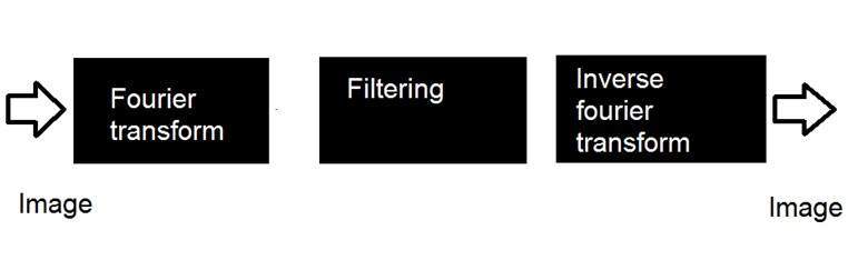
The steps in filtering are given below.
At first step we have to do some pre – processing an image in spatial domain, means increase its contrast or brightness
Then we will take discrete Fourier transform of the image
Then we will center the discrete Fourier transform , as we will bring the discrete Fourier transform in center from corners
Then we will apply filtering , means we will multiply the Fourier transform by a filter function
Then we will again shift the DFT from center to the corners
Last step would be take to inverse discrete Fourier transform , to bring the result back from frequency domain to spatial domain
And this step of post processing is optional , just like pre processing , in which we just increase the appearance of image.
Filters
The concept of filter in frequency domain is same as the concept of a mask in convolution.
After converting an image to frequency domain, some filters are applied in filtering process to perform different kind of processing on an image. The processing include blurring an image , sharpening an image e.t.c.
The common type of filters for these purposes are:
Ideal high pass filter
Ideal low pass filter
Gaussian high pass filter
Gaussian low pass filter
In the next tutorial, we will discuss about filter in detail.
High Pass vs Low Pass Filters
In the last tutorial , we briefly discuss about filters. In this tutorial we will thoroughly discuss about them. Before discussing about let’s talk about masks first. The concept of mask has been discussed in our tutorial of convolution and masks.
Blurring masks vs derivative masks.
We are going to perform a comparison between blurring masks and derivative masks.
Blurring masks:
A blurring mask has the following properties.
All the values in blurring masks are positive
The sum of all the values is equal to 1
The edge content is reduced by using a blurring mask
As the size of the mask grow, more smoothing effect will take place
Derrivative masks:
A derivative mask has the following properties.
A derivative mask have positive and as well as negative values
The sum of all the values in a derivative mask is equal to zero
The edge content is increased by a derivative mask
As the size of the mask grows , more edge content is increased
Relationship between blurring mask and derivative mask with high pass filters and low pass filters.
The relationship between blurring mask and derivative mask with a high pass filter and low pass filter can be defined simply as.
Blurring masks are also called as low pass filter
Derivative masks are also called as high pass filter
High pass frequency components and Low pass frequency components
The high pass frequency components denotes edges whereas the low pass frequency components denotes smooth regions.
Ideal low pass and Ideal High pass filters
This is the common example of low pass filter.
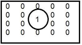
When one is placed inside and the zero is placed outside , we got a blurred image. Now as we increase the size of 1, blurring would be increased and the edge content would be reduced.
This is a common example of high pass filter.
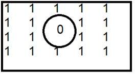
When 0 is placed inside, we get edges , which gives us a sketched image. An ideal low pass filter in frequency domain is given below
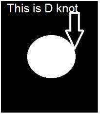
The ideal low pass filter can be graphically represented as
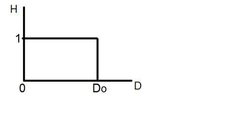
Now let’s apply this filter to an actual image and let’s see what we got.
Sample image.

Image in frequency domain
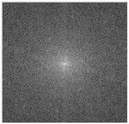
Applying filter over this image
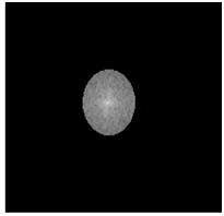
Resultant Image

With the same way , an ideal high pass filter can be applied on an image. But obviously the results would be different as , the low pass reduces the edged content and the high pass increase it.
Gaussian Low pass and Gaussian High pass filter
Gaussian low pass and Gaussian high pass filter minimize the problem that occur in ideal low pass and high pass filter.
This problem is known as ringing effect. This is due to reason because at some points transition between one color to the other cannot be defined precisely, due to which the ringing effect appears at that point.
Have a look at this graph.

This is the representation of ideal low pass filter. Now at the exact point of Do , you cannot tell that the value would be 0 or 1. Due to which the ringing effect appears at that point.
So in order to reduce the effect that appears is ideal low pass and ideal high pass filter , the following Gaussian low pass filter and Gaussian high pass filter is introduced.
Gaussian Low pass filter
The concept of filtering and low pass remains the same, but only the transition becomes different and become more smooth.
The Gaussian low pass filter can be represented as
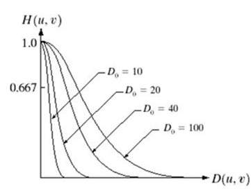
Note the smooth curve transition, due to which at each point, the value of Do , can be exactly defined.
Gaussian high pass filter
Gaussian high pass filter has the same concept as ideal high pass filter , but again the transition is more smooth as compared to the ideal one.
Introduction to Color Spaces
In this tutorial, we are going to talk about color spaces.
What are color spaces?
Color spaces are different types of color modes, used in image processing and signals and system for various purposes. Some of the common color spaces are:
RGB
CMY’K
Y’UV
YIQ
Y’CbCr
HSV
RGB
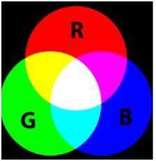
RGB is the most widely used color space , and we have already discussed it in the past tutorials. RGB stands for red green and blue.
What RGB model states , that each color image is actually formed of three different images. Red image , Blue image , and black image. A normal grayscale image can be defined by only one matrix, but a color image is actually composed of three different matrices.
One color image matrix = red matrix + blue matrix + green matrix
This can be best seen in this example below.
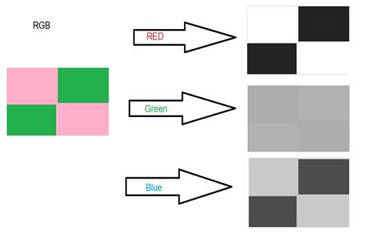
Applications of RGB
The common applications of RGB model are
Cathode ray tube (CRT)
Liquid crystal display (LCD)
Plasma Display or LED display such as a television
A compute monitor or a large scale screen
CMYK
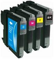
RGB to CMY conversion
The conversion from RGB to CMY is done using this method.
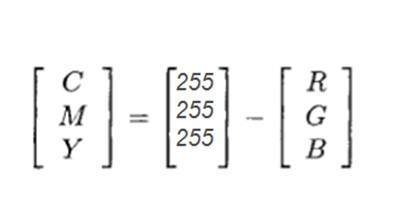
Consider you have an color image , means you have three different arrays of RED , GREEN and BLUE. Now if you want to convert it into CMY , here’s what you have to do. You have to subtract it by the maximum number of levels – 1. Each matrix is subtracted and its respective CMY matrix is filled with result.
Y’UV
Y’UV defines a color space in terms of one luma (Y’) and two chrominance (UV) components. The Y’UV color model is used in the following composite color video standards.
NTSC ( National Television System Committee)
PAL (Phase Alternating Line)
SECAM (Sequential couleur a amemoire, French for “sequential color with memory)
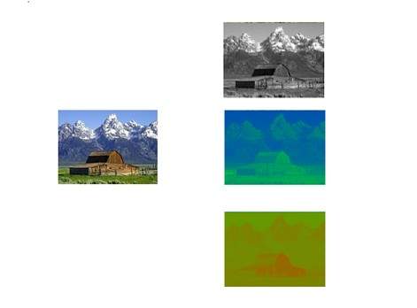
Y’CbCr
Y’CbCr color model contains Y’ , the luma component and cb and cr are the blue-differnece and red difference chroma components.
It is not an absolute color space. It is mainly used for digital systems
Its common applications include JPEG and MPEG compression.
Y’UV is often used as the term for Y’CbCr, however they are totally different formats. The main difference between these two is that the former is analog while the later is digital.
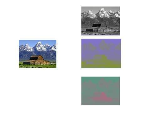
Introduction to JPEG Compression
In our last tutorial of image compression , we discuss some of the techniques used for compression
We are going to discuss JPEG compression which is lossy compression , as some data is loss in the end.
Let’s discuss first what image compression is.
Image compression
Image compression is the method of data compression on digital images.
The main objective in the image compression is:
Store data in an efficient form
Transmit data in an efficient form
Image compression can be lossy or lossless.
JPEG compression
JPEG stands for Joint photographic experts group. It is the first interanational standard in image compression. It is widely used today. It could be lossy as well as lossless . But the technique we are going to discuss here today is lossy compression technique.
How jpeg compression works:
First step is to divide an image into blocks with each having dimensions of 8 x8.
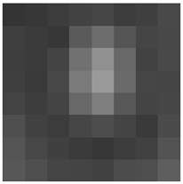
Let’s for the record , say that this 8x8 image contains the following values.
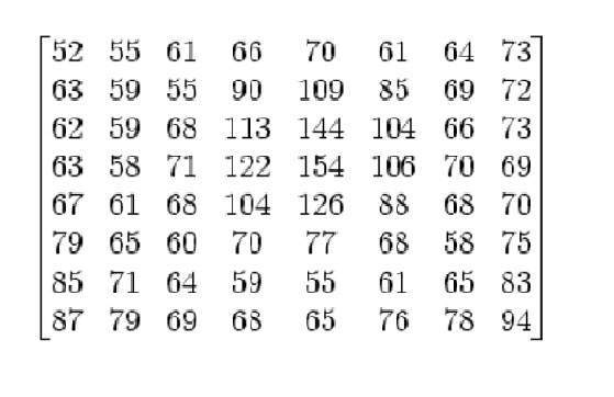
The range of the pixels intensities now are from 0 to 255. We will change the range from -128 to 127.
Subtracting 128 from each pixel value yields pixel value from -128 to 127. After subtracting 128 from each of the pixel value , we got the following results.
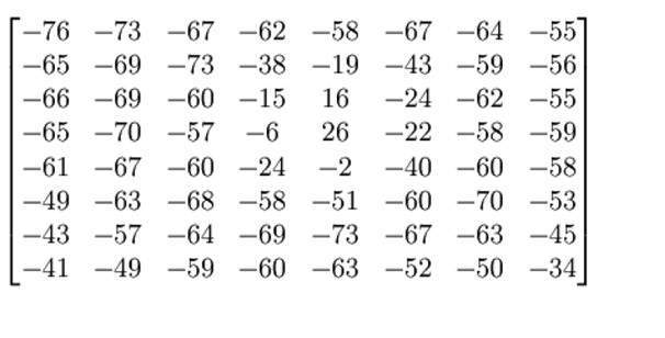
Now we will compute using this formula.
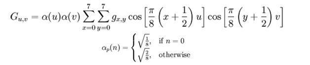
The result comes from this is stored in let’s say A(j,k) matrix.
There is a standard matrix that is used for computing JPEG compression, which is given by a matrix called as Luminance matrix.
This matrix is given below
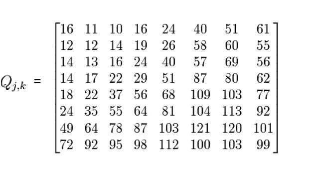
Applying the following formula
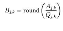
We got this result after applying.
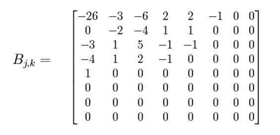
Now we will perform the real trick which is done in JPEG compression which is ZIG-ZAG movement. The zig zag sequence for the above matrix is shown below. You have to perform zig zag until you find all zeroes ahead. Hence our image is now compressed.
Summarizing JPEG compression
The first step is to convert an image to Y’CbCr and just pick the Y’ channel and break into 8 x 8 blocks. Then starting from the first block , map the range from -128 to 127. After that you have to find the discrete fourier transform of the matrix. The result of this should be quantized. The last step is to apply encoding in the zig zag manner and do it till you find all zero.
Save this one dimensional array and you are done.
Note. You have to repeat this procedure for all the block of 8 x 8.
Optical Character Recognition
Optical character recognition is usually abbreviated as OCR. It includes the mechanical and electrical conversion of scanned images of handwritten, typewritten text into machine text. It is common method of digitizing printed texts so that they can be electronically searched, stored more compactly, displayed on line, and used in machine processes such as machine translation, text to speech and text mining.
In recent years, OCR (Optical Character Recognition) technology has been applied throughout the entire spectrum of industries, revolutionizing the document management process. OCR has enabled scanned documents to become more than just image files, turning into fully searchable documents with text content that is recognized by computers. With the help of OCR, people no longer need to manually retype important documents when entering them into electronic databases. Instead, OCR extracts relevant information and enters it automatically. The result is accurate, efficient information processing in less time.
Optical character recognition has multiple research areas but the most common areas are as following:
Banking:
he uses of OCR vary across different fields. One widely known application is in banking, where OCR is used to process checks without human involvement. A check can be inserted into a machine, the writing on it is scanned instantly, and the correct amount of money is transferred. This technology has nearly been perfected for printed checks, and is fairly accurate for handwritten checks as well, though it occasionally requires manual confirmation. Overall, this reduces wait times in many banks.
Blind and visually impaired persons:
One of the major factors in the beginning of research behind the OCR is that scientist want to make a computer or device which could read book to the blind people out loud. On this research scientist made flatbed scanner which is most commonly known to us as document scanner.
Legal department:
In the legal industry, there has also been a significant movement to digitize paper documents. In order to save space and eliminate the need to sift through boxes of paper files, documents are being scanned and entered into computer databases. OCR further simplifies the process by making documents text-searchable, so that they are easier to locate and work with once in the database. Legal professionals now have fast, easy access to a huge library of documents in electronic format, which they can find simply by typing in a few keywords.
Retail Industry:
Barcode recognition technology is also related to OCR. We see the use of this technology in our common day use.
Other Uses:
OCR is widely used in many other fields, including education, finance, and government agencies. OCR has made countless texts available online, saving money for students and allowing knowledge to be shared. Invoice imaging applications are used in many businesses to keep track of financial records and prevent a backlog of payments from piling up. In government agencies and independent organizations, OCR simplifies data collection and analysis, among other processes. As the technology continues to develop, more and more applications are found for OCR technology, including increased use of handwriting recognition.
Computer Vision and Computer Graphics
Computer Vision
Computer vision is concerned with modeling and replicating human vision using computer software and hardware. Formally if we define computer vision then its definition would be that computer vision is a discipline that studies how to reconstruct, interrupt and understand a 3d scene from its 2d images in terms of the properties of the structure present in scene.
It needs knowledge from the following fields in order to understand and stimulate the operation of human vision system.
Computer Science
Electrical Engineering
Mathematics
Physiology
Biology
Cognitive Science
Computer Vision Hierarchy:
Computer vision is divided into three basic categories that are as following:
Low-level vision: includes process image for feature extraction.
Intermediate-level vision: includes object recognition and 3D scene Interpretation
High-level vision: includes conceptual description of a scene like activity, intention and behavior.
Related Fields:
Computer Vision overlaps significantly with the following fields:
Image Processing: it focuses on image manipulation.
Pattern Recognition: it studies various techniques to classify patterns.
Photogrammetry: it is concerned with obtaining accurate measurements from images.
Computer Vision Vs Image Processing:
Image processing studies image to image transformation. The input and output of image processing are both images.
Computer vision is the construction of explicit, meaningful descriptions of physical objects from their image. The output of computer vision is a description or an interpretation of structures in 3D scene.
Example Applications:
Robotics
Medicine
Security
Transportation
Industrial Automation
Robotics Application:
Localization-determine robot location automatically
Navigation
Obstacles avoidance
Assembly (peg-in-hole, welding, painting)
Manipulation (e.g. PUMA robot manipulator)
Human Robot Interaction (HRI): Intelligent robotics to interact with and serve people
Medicine Application:
Classification and detection (e.g. lesion or cells classification and tumor detection)
2D/3D segmentation
3D human organ reconstruction (MRI or ultrasound)
Vision-guided robotics surgery
Industrial Automation Application:
Industrial inspection (defect detection)
Assembly
Barcode and package label reading
Object sorting
Document understanding (e.g. OCR)
Security Application:
Biometrics (iris, finger print, face recognition)
Surveillance-detecting certain suspicious activities or behaviors
Transportation Application:
Autonomous vehicle
Safety, e.g., driver vigilance monitoring
Computer Graphics
Computer graphics are graphics created using computers and the representation of image data by a computer specifically with help from specialized graphic hardware and software. Formally we can say that Computer graphics is creation, manipulation and storage of geometric objects (modeling) and their images (Rendering).
The field of computer graphics developed with the emergence of computer graphics hardware. Today computer graphics is use in almost every field. Many powerful tools have been developed to visualize data. Computer graphics field become more popular when companies started using it in video games. Today it is a multibillion dollar industry and main driving force behind the computer graphics development. Some common applications areas are as following:
Computer Aided Design (CAD)
Presentation Graphics
3d Animation
Education and training
Graphical User Interfaces
Computer Aided Design:
Used in design of buildings, automobiles, aircraft and many other product
Use to make virtual reality system.
Presentation Graphics:
Commonly used to summarize financial ,statistical data
Use to generate slides
3d Animation:
Used heavily in the movie industry by companies such as Pixar, DresmsWorks
To add special effects in games and movies.
Education and training:
Computer generated models of physical systems
Medical Visualization
3D MRI
Dental and bone scans
Stimulators for training of pilots etc.
Graphical User Interfaces:
It is used to make graphical user interfaces objects like buttons, icons and other components